An introduction to modeltuner with examples

library(modeltuner)
library(magrittr, warn.conflicts = FALSE)   # for pipe operator
options(cv_verbose = FALSE, width = 100)

Basics

The package modeltuner offers a toolkit for model evaluation, model comparison and hyperparameter tuning based on cross-validation. It applies to models for a continuous or binary response that are generated with the formula interface. In addition, it includes functionalities for conveniently fitting and tuning xgboost and glmnet models.

The formula interface

modeltuner is designed for model classes that are based on a model-fitting functions using the formula interface in combination with a data argument. Examples of model-fitting functions matching this requirement are:

in package stats: lm(), glm(), loess(), nls()
in package robustbase: lmrob(), glmrob(), nlrob()
in package MASS: rlm(), lqs()
in package mgcv: gam()
in package rpart: rpart()
in package quantreg: rq()
in package lme4: lmer(), glmer()

modeltuner adds a few functions to this list which are essentially formula-based wrappers to functions not supporting the formula interface:

fm_smoothing_spline() uses stats::smooth.spline(),
fm_knn() uses RANN::nn2() (nearest-neighbor),
fm_xgb() uses xgboost::xgb.train()
fm_glmnet() uses glmnet::glmnet()

The package offers some particularly attractive tools for handling what is called iteratively fitted models (IFM) here. For such a model, the fitting process returns not just one single model (or model parameterization), but rather a range of models (or model parameterizations) of increasing structural complexity. Prominent examples –and currently the only instances implemented in the package– are gradient boosting (as implemented in package xgboost) and Lasso regression and elastic nets (available from package glmnet). Refer to the dedicated vignette (vignette("ifm")) for an overview of these functionalities.

Fitted models and objects of class “model”

We use the term fitted model for the output of a model-fitting function, such as lm(). In modeltuner, models are alternatively represented as objects of class “model”. Such a “model” object does not necessarily contain the model fit, but it includes the information needed to refit the model, notably the model fitting call and the complete data.

Each model has a label used to identify it in printed output and graphics, in particular when several models are compared. The default label is "model", but it is recommended to attribute an informative label to each model you create.

fm_lm_cars <- lm(dist ~ speed, cars)        # fitted model
mod_lm_cars <- model(fm_lm_cars, label = "lm_cars") # 'model' object
mod_lm_cars

## --- A "model" object ---
##   label:          lm_cars
##   model class:    lm
##   formula:        dist ~ speed
##   data:           data.frame [50 x 2], input as: 'data = cars'
##   response_type:  continuous
##   call:           lm(formula = dist ~ speed, data = data)
##   fit:            Object of class 'lm'

class(mod_lm_cars)

## [1] "model_lm" "model"

Note the generic setting data=data in the model generating call of model_lm_cars in the printed output above. This is convenient for cross-validation, where the model generating call is repeatedly adjusted and executed internally, using the data stored in the “model” object. A similar generic setting weights=weights is imposed in case of a weighted model.

In order to obtain the fitted model corresponding to a given “model” object, use fit(). In a sense, fit() is the reverse operation of model(). fit(mod_lm_cars) essentially executes the call mod_lm_cars$call using the data mod_lm_cars$data.

fit(mod_lm_cars)    # back to fitted models

## 
## Call:
## lm(formula = dist ~ speed, data = cars)
## 
## Coefficients:
## (Intercept)        speed  
##     -17.579        3.932

all.equal(fm_lm_cars, fit(mod_lm_cars))

## [1] TRUE

Cross validation

Folds

The function make_folds() generates a set of groups for cross validation, sometimes called “folds”. Its output essentially consists in a list of integer vectors defining the test sets. The complement of each test set is used as the corresponding training set.

make_folds(cars)              # 10-fold CV, the default

## Validation procedure: Complete k-fold Cross-Validation
##   Number of obs in data:  50
##   Number of test sets:    10
##   Size of test sets:       5
##   Size of training sets:  45

str(make_folds(cars))

## List of 10
##  $ : int [1:5] 15 18 31 34 36
##  $ : int [1:5] 16 33 39 40 45
##  $ : int [1:5] 11 24 25 42 47
##  $ : int [1:5] 6 10 21 30 49
##  $ : int [1:5] 3 4 13 28 38
##  $ : int [1:5] 2 7 29 43 50
##  $ : int [1:5] 14 20 22 23 48
##  $ : int [1:5] 8 9 27 32 35
##  $ : int [1:5] 1 5 12 17 44
##  $ : int [1:5] 19 26 37 41 46
##  - attr(*, "class")= chr [1:2] "folds" "list"
##  - attr(*, "type")= chr "complete"
##  - attr(*, "n")= int 50
##  - attr(*, "stratified")= logi FALSE

Using the argument nfold to create 5-fold cross-validation:

make_folds(cars, nfold = 5)

## Validation procedure: Complete k-fold Cross-Validation
##   Number of obs in data:  50
##   Number of test sets:     5
##   Size of test sets:      10
##   Size of training sets:  40

Setting nfold=p with a value of p between 0 and 1 is also possible. Instead of a cross-validation, this evokes a simple hold-out validation, where the model is fitted to the proportion $(1-p) \cdot 100\%$ of the data and the remaining $p \cdot 100\%$ is used for evaluation.

make_folds(cars, nfold = 0.3) # Simple hold-out validation with 30% of cases in test set

## Validation procedure: Simple Hold-out Validation
##   Number of obs in data:  50
##   Number of test sets:     1
##   Size of test set:       15
##   Size of training set:   35

Execute a cross-validation: `cv()`

make_folds() is used inside cv(), the core function executing a cross-validation. By default, 10-fold CV is performed, but this can be customized using arguments nfold and folds,

# Executing a cross validation: cv()
cv_cars <- cv(mod_lm_cars)
cv_cars

## --- A "cv" object containing 1 validated model ---
## 
## Validation procedure: Complete k-fold Cross-Validation
##   Number of obs in data:  50
##   Number of test sets:    10
##   Size of test sets:       5
##   Size of training sets:  45
## 
## Model:
## 
## 'lm_cars':
##   model class:  lm
##   formula:      dist ~ speed
##   metric:       rmse

cv() can also be applied directly to a fitted model: cv(fm_lm_cars) executes fm_lm_cars %>% model %>% cv, thus skipping the model step. The method used in this case is cv.default().

Evaluate a cross-validation: `cv_performance()`

To evaluate a “cv” object, use cv_performance():

cv_performance(cv_cars)

## --- Performance table ---
## Metric: rmse
##         train_rmse test_rmse time_cv
## lm_cars     15.013    14.812    0.01

cv_performance(cv_cars, metric = "medae") # alternative metric, see ?metrics

## --- Performance table ---
## Metric: medae
##         train_medae test_medae time_cv
## lm_cars      9.9791     10.739    0.01

There are so-called “shortcut methods” of cv_perrormance() that trigger several steps in the workflow sketched above. Examples are cv_performance.model() or cv_performance.default().

cv_performance.model(x) executes x %>% cv %>% cv_performance:

cv_performance(mod_lm_cars)

## --- Performance table ---
## Metric: rmse
##         train_rmse test_rmse time_cv
## lm_cars     15.002    14.395   0.009

The method cv_performance.default is applied to a fitted model and executes x %>% model %>% cv %>% cv_performance:

cv_performance(fm_lm_cars)     # cv_performance.default - applied to a fitted model

## --- Performance table ---
## Metric: rmse
##       train_rmse test_rmse time_cv
## model      14.99    14.815   0.009

A drawback of these shortcut methods is that potentially useful interim results from cross-validation (the “cv” object) is not being stored. It is useful to know that the result from the last execution of cv() can be recovered at any time with last_cv().

Saving the model fits

By default, the model fits from a cross validation are not saved. To do so, set keep_fits = TRUE in cv():

Keep the fitted models from the cross-validation:

cv_cars_fits <- cv(mod_lm_cars, keep_fits = T)

extract_fits() can now be used to obtain the model fits from a “cv” object. Besides the model fits, the resulting table also has column containing the folds.

(cars_fits <- extract_fits(cv_cars_fits))

##       folds lm_cars
## 1  <int>[5]    <lm>
## 2  <int>[5]    <lm>
## 3  <int>[5]    <lm>
## 4  <int>[5]    <lm>
## 5  <int>[5]    <lm>
## 6  <int>[5]    <lm>
## 7  <int>[5]    <lm>
## 8  <int>[5]    <lm>
## 9  <int>[5]    <lm>
## 10 <int>[5]    <lm>

We could now extract the fitted coefficients of the 10 models as follows:

sapply(cars_fits$lm_cars, coef)

##                   [,1]       [,2]       [,3]       [,4]       [,5]       [,6]       [,7]       [,8]
## (Intercept) -16.434962 -18.297725 -21.183227 -13.892332 -17.339967 -18.314134 -17.175287 -19.644122
## speed         3.916652   4.000578   4.265483   3.634229   3.916122   3.969363   3.847343   3.999979
##                   [,9]      [,10]
## (Intercept) -14.096414 -19.856576
## speed         3.731144   4.068375

Multimodels

A multimodel combines several models in one object. In order to create such a multimodel, we fit two alternative models to the cars data.

Alternative model 1: LOESS (locally weighted polynomial regression) with stats::loess():

fm_loess_cars <- loess(dist ~ speed, cars,  
      control = loess.control(surface = "direct"))

(The control setting in loess() is necessary for predictions outside of the range of the training data)

Alternative model 2: regression tree with rpart::rpart():

fm_rpart_cars <- rpart::rpart(dist ~ speed, cars)

These three models are combined in a multimodel with the method c.model():

mm_cars <- c(  # method c.model(): argument names are used as model labels
  lm = model(fm_lm_cars), 
  loess = model(fm_loess_cars), 
  rpart = model(fm_rpart_cars))
mm_cars

## --- A "multimodel" object containing 3 models ---
## 
## 'lm':
##   model class:  lm
##   formula:      dist ~ speed
##   data:         data.frame [50 x 2], input as: 'data = cars'
##   call:         lm(formula = dist ~ speed, data = data)
## 
## 'loess':
##   model class:  loess
##   formula:      dist ~ speed
##   data:         data.frame [50 x 2], input as: 'data = cars'
##   call:         loess(formula = dist ~ speed, data = data, control = loess.control(surface = "direct"))
## 
## 'rpart':
##   model class:  rpart
##   formula:      dist ~ speed
##   data:         data.frame [50 x 2], input as: 'data = cars'
##   call:         rpart::rpart(formula = dist ~ speed, data = data)

Only models having the same response can be combined in a multimodel.

Graphical illustration of the fits of the three models:

library(ggplot2, warn.conflicts = F)
speed_seq <- seq(0, 30, .1)  # grid of data points along range of 'speed'
preds_mm <- predict(mm_cars, data.frame(speed = speed_seq)) # predictions for grid data
preds_mm <- data.frame(  # reshape for ggplot
  speed = rep(speed_seq, 3),
  model = rep(label(mm_cars), each = length(speed_seq)), 
  dist = as.vector(preds_mm))
ggplot(preds_mm, aes(speed, dist, color = model)) +
  geom_point(data = cars, color = 8) +
  geom_line(lwd = 1) +
  ggtitle("cars data: comparison of model fits")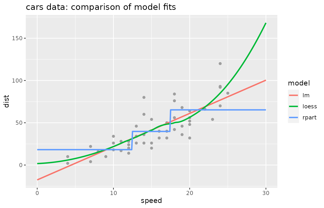

Cross-validate a multimodel

cv() and cv_performance() are applied to a multimodel exactly as to a model. The same set of folds is thereby used for all three cross-validations.

cv_cars <- cv(mm_cars)
cv_performance(cv_cars)

## --- Performance table ---
## Metric: rmse
##       train_rmse test_rmse time_cv
## lm        15.021    14.228   0.009
## loess     14.277    14.529   0.167
## rpart     16.513    15.948   0.019

The output of cv(), an object of class “cv”, has a plot() method producing a scatter plot of response versus predicted values using the out-of-sample predictions resulting from the cross-validation.

plot(cv_cars)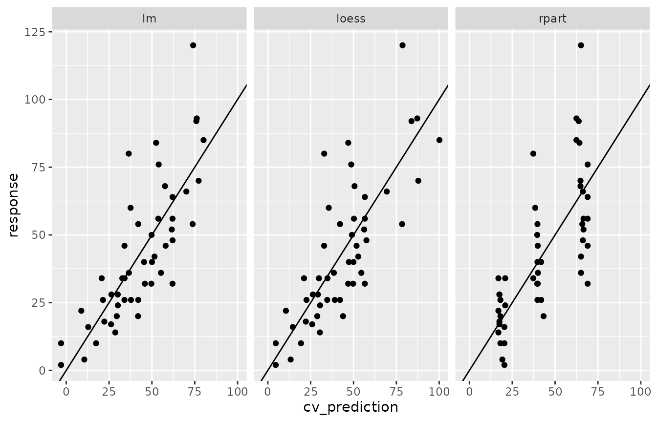

Find the best-fitting model: `tune()`

tune() applied to a “cv” object extracts the best fitting model according to test performance.

# tune: pick the best model
tune(cv_cars)

## --- A "model" object ---
##   label:          lm
##   model class:    lm
##   formula:        dist ~ speed
##   data:           data.frame [50 x 2], input as: 'data = cars'
##   response_type:  continuous
##   call:           lm(formula = dist ~ speed, data = data)
##   fit:            Object of class 'lm'

tune(cv_cars) %>% fit  # back to fitted model

## 
## Call:
## lm(formula = dist ~ speed, data = cars)
## 
## Coefficients:
## (Intercept)        speed  
##     -17.579        3.932

If applied to a multimodel, tune() will cross-validate the multimodel and then return the best-fitting model. Different runs of cv() use different folds and consequently yield varying results, such that the “best” model picked by tune() can vary, too. In order to impose a given set of folds, use the parameter folds in cv():

cv(mm_cars, folds = cv_cars$folds) %>% cv_performance  # Same results as cv_performance(cv_cars)

## --- Performance table ---
## Metric: rmse
##       train_rmse test_rmse time_cv
## lm        15.021    14.228   0.014
## loess     14.277    14.529   0.011
## rpart     16.513    15.948   0.018

cv(mm_cars) %>% cv_performance   # Slightly different results

## --- Performance table ---
## Metric: rmse
##       train_rmse test_rmse time_cv
## lm        15.040    14.754   0.009
## loess     14.319    14.995   0.011
## rpart     16.237    16.812   0.018

The modeltuner package comes with a number of generic utility functions that are helpful for inspection and basic manipulations of object of classes “model”, “multimodel”, “cv”, “performance” (the output of cv_performance()) and other. Some of these are presented in this section.

Number of models and model labels: `n_model()`, `label()`

Query the number of models in mm_cars and their labels:

n_model(mm_cars)

## [1] 3

label(mm_cars)

## [1] "lm"    "loess" "rpart"

Modify model labels: label<- or set_labels()

set_label(mm_cars, c("m1", "m2", "m3"))  # or:  label(mm_cars) <- c("m1", "m2", "m3")

## --- A "multimodel" object containing 3 models ---
## 
## 'm1':
##   model class:  lm
##   formula:      dist ~ speed
##   data:         data.frame [50 x 2], input as: 'data = cars'
##   call:         lm(formula = dist ~ speed, data = data)
## 
## 'm2':
##   model class:  loess
##   formula:      dist ~ speed
##   data:         data.frame [50 x 2], input as: 'data = cars'
##   call:         loess(formula = dist ~ speed, data = data, control = loess.control(surface = "direct"))
## 
## 'm3':
##   model class:  rpart
##   formula:      dist ~ speed
##   data:         data.frame [50 x 2], input as: 'data = cars'
##   call:         rpart::rpart(formula = dist ~ speed, data = data)

The parameter which allows changing only a part of the labels:

set_label(mm_cars, which = 3, "tree")    # changes only the third label (result not shown)

Subsetting a multimodel or “cv” object with `subset()`

subset.multimodel() subsets a multimodel. The selection can be made with an integer, character (giving model labels) or logical (of appropriate length) vector.

subset(mm_cars, c(1, 3))  # i is integer

## --- A "multimodel" object containing 2 models ---
## 
## 'lm':
##   model class:  lm
##   formula:      dist ~ speed
##   data:         data.frame [50 x 2], input as: 'data = cars'
##   call:         lm(formula = dist ~ speed, data = data)
## 
## 'rpart':
##   model class:  rpart
##   formula:      dist ~ speed
##   data:         data.frame [50 x 2], input as: 'data = cars'
##   call:         rpart::rpart(formula = dist ~ speed, data = data)

subset(mm_cars, c("lm", "rpart")) # i is character - same result as above
subset(mm_cars, c(T, F, T))       # i is logical - same result as above

The methods subset.cv() and subset.performance() work analogously.

Extraction of a model from a multimodel or “cv” object: `extract_model()`

While subset.cv() yields another “cv” object, extract_model() extracts a single model from a “cv” object or multimodel, returning an object of class “model”.

# extract the first model
extract_model(cv_cars, 1)  # i (second argument) is integer

## --- A "model" object ---
##   label:          lm
##   model class:    lm
##   formula:        dist ~ speed
##   data:           data.frame [50 x 2], input as: 'data = cars'
##   response_type:  continuous
##   call:           lm(formula = dist ~ speed, data = data)
##   fit:            Object of class 'lm'

extract_model(cv_cars, "lm")       # i is character - same result as above
extract_model(cv_cars, c(T, F, F)) # i is logical - same result as above

Note that there is also a function extract_multimodel(), which extracts the multimodel from a “cv” object.

Sort the models: `sort_models()`

# sort models
sort_models(mm_cars, c(1, 3, 2))

## --- A "multimodel" object containing 3 models ---
## 
## 'lm':
##   model class:  lm
##   formula:      dist ~ speed
##   data:         data.frame [50 x 2], input as: 'data = cars'
##   call:         lm(formula = dist ~ speed, data = data)
## 
## 'rpart':
##   model class:  rpart
##   formula:      dist ~ speed
##   data:         data.frame [50 x 2], input as: 'data = cars'
##   call:         rpart::rpart(formula = dist ~ speed, data = data)
## 
## 'loess':
##   model class:  loess
##   formula:      dist ~ speed
##   data:         data.frame [50 x 2], input as: 'data = cars'
##   call:         loess(formula = dist ~ speed, data = data, control = loess.control(surface = "direct"))

sort_models(mm_cars, c(1, 3))  # same as above (omitted index 2 is appended)

Sorting by performance and execution time is also possible:

cv_performance(cv_cars) %>% sort_models(by = "test") # not for multimodels

## --- Performance table ---
## Metric: rmse
##       train_rmse test_rmse time_cv
## lm        15.021    14.228   0.009
## loess     14.277    14.529   0.167
## rpart     16.513    15.948   0.019

cv_performance(cv_cars) %>% sort_models(by = "time") # not for multimodels

## --- Performance table ---
## Metric: rmse
##       train_rmse test_rmse time_cv
## lm        15.021    14.228   0.009
## rpart     16.513    15.948   0.019
## loess     14.277    14.529   0.167

n_model(), label(), label<-, set_label(), subset(), extract_model(), sort_model() have specific methods for classes “model”, “multimodel”, “cv” and “performance”. Their help topics have more detailed information.

Hyperparameter tuning

Motivating example: Parameter `k` in k-nearest-neighbor

We now use the function fm_knn() (from the modeltuner package) to fit a k-nearest model to the mycycle data from package MASS. The parameter k, the number of neighbors, equals 5 by default.

data(mcycle, package = "MASS")

fm_mcycle <- fm_knn(accel ~ times, data = mcycle) # function from modeltuner; k=5 by default
fm_mcycle

## k-nearest neighbors model (class 'fm_knn')
##   formula:      accel ~ times - 1
##   data:         mcycle
##   k:            5
##   n:            133
##   standardize:  TRUE
##   weighted:     FALSE

Illustration of the model fit:

# First create a grid along the range of 'times' (used for graphs)
preddat <- data.frame(times = with(mcycle, seq(min(times), max(times), length.out = 100)))
preddat$accel <- predict(fm_mcycle, preddat)
ggplot(preddat, aes(times, accel)) +
  geom_hline(yintercept = 0, lty = 3) +
  geom_line(col = 2, lwd = 1) +
  geom_point(data = mcycle, col = 4, alpha = 0.5)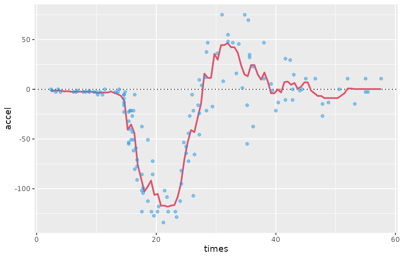

Create a multimodel with `multimodel()`

Next, a multimodel is generated that contains 25 “fm_knn”-models with different choices of the parameter k:

kk <- 1:25
knn_mcycle <- multimodel(fm_mcycle, k = kk, prefix = "knn_mcycle")
knn_mcycle

## --- A "multimodel" object containing 25 models ---
## 
## 'knn_mcycle1':
##   model class:  fm_knn
##   formula:      accel ~ times
##   data:         data.frame [133 x 2], input as: 'data = mcycle'
##   call:         fm_knn(formula = accel ~ times, data = data, k = 1L)
## 
## 'knn_mcycle2':
##   model class:  fm_knn
##   formula:      accel ~ times
##   data:         data.frame [133 x 2], input as: 'data = mcycle'
##   call:         fm_knn(formula = accel ~ times, data = data, k = 2L)
## 
## 'knn_mcycle3':
##   model class:  fm_knn
##   formula:      accel ~ times
##   data:         data.frame [133 x 2], input as: 'data = mcycle'
##   call:         fm_knn(formula = accel ~ times, data = data, k = 3L)
## 
## and 22 models more, labelled:
##   'knn_mcycle4', 'knn_mcycle5', 'knn_mcycle6', 'knn_mcycle7', 'knn_mcycle8', 'knn_mcycle9', 
##   'knn_mcycle10', 'knn_mcycle11', 'knn_mcycle12', 'knn_mcycle13', 'knn_mcycle14', 'knn_mcycle15', 
##   'knn_mcycle16', 'knn_mcycle17', 'knn_mcycle18', 'knn_mcycle19', 'knn_mcycle20', 'knn_mcycle21', 
##   'knn_mcycle22', 'knn_mcycle23', 'knn_mcycle24', 'knn_mcycle25'
## 
## 
## Parameter table:
##               k
## knn_mcycle1   1
## knn_mcycle2   2
## knn_mcycle3   3
## ... 22 rows omitted (nrow=25)

As opposed to a multimodel obtained by joining several model with c(...), a multimodel generated with multimodel() has a parameter table that is displayed when the multimodel is printed, see the output above.

The multimodel mm_cycle is cross-validated:

cv_mcycle <- cv(knn_mcycle) # Uses same folds for all models
cv_performance(cv_mcycle)

## --- Performance table ---
## Metric: rmse
##               k train_rmse test_rmse time_cv
## knn_mcycle1   1     17.622    33.649   0.016
## knn_mcycle2   2     18.214    27.984   0.015
## knn_mcycle3   3     19.671    26.292   0.016
## knn_mcycle4   4     20.202    25.751   0.016
## knn_mcycle5   5     20.397    25.726   0.016
## knn_mcycle6   6     20.868    25.071   0.017
## knn_mcycle7   7     21.178    25.116   0.016
## knn_mcycle8   8     21.358    24.644   0.016
## knn_mcycle9   9     21.781    24.611   0.016
## knn_mcycle10 10     22.027    24.691   0.017
## knn_mcycle11 11     22.177    24.594   0.016
## knn_mcycle12 12     22.297    24.691   0.018
## knn_mcycle13 13     22.479    24.654   0.018
## knn_mcycle14 14     22.618    24.437   0.018
## knn_mcycle15 15     22.865    24.689   0.017
## knn_mcycle16 16     23.080    24.658   0.018
## knn_mcycle17 17     23.290    24.732   0.018
## knn_mcycle18 18     23.518    25.060   0.027
## knn_mcycle19 19     23.816    25.436   0.017
## knn_mcycle20 20     24.136    25.404   0.017
## knn_mcycle21 21     24.391    25.546   0.017
## knn_mcycle22 22     24.699    26.009   0.018
## knn_mcycle23 23     25.031    26.311   0.018
## knn_mcycle24 24     25.520    26.664   0.017
## knn_mcycle25 25     25.932    27.045   0.018

Note that the column(s) of the parameter table, k in our example, are included in the output of cv_performance().

Plot a performance table

The output of cv_performance() is a performance table, of class “performance”. Its plot() method displays a bar chart by default.

cv_performance(cv_mcycle) %>% plot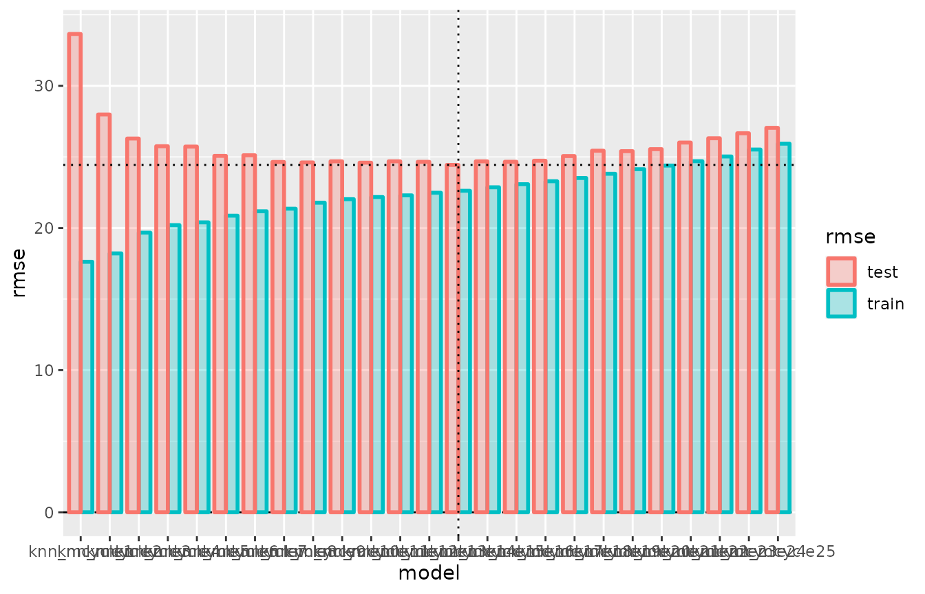

The vertical dotted line identifies the best-fitting model (w.r.t. test error), i.e. the model that tune() would pick. The horizontal dotted line shows the test error of this model.

In this example, the visual appearance of the plot can be improved by setting the parameter xvar:

cv_performance(cv_mcycle) %>% plot(xvar = "k") # xvar a column of the performance table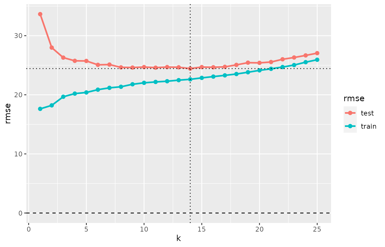

Note that the training error of the 1-nearest neighbor model is larger than zero. This is due to the presence of bindings mcycle$times. Without bindings, the curve representing the training error would start at a value of zero.

The next plot compares the model fits for a custom selection of four values of k:

preds <- predict(subset(knn_mcycle, c(1, 5, 10, 25)), preddat)
data.frame(
  model = factor(rep(colnames(preds), each = nrow(preds)), 
                 levels = paste0("knn_mcycle", c(1, 5, 10, 25))),
  times = preddat$times, 
  accel = as.vector(preds)) %>% 
  ggplot(aes(times, accel)) +
  facet_wrap(~ model) +
  geom_hline(yintercept = 0, lty = 3) +
  geom_line(col = 2, lwd = 1) +
  geom_point(data = mcycle, col = 4, alpha = 0.5)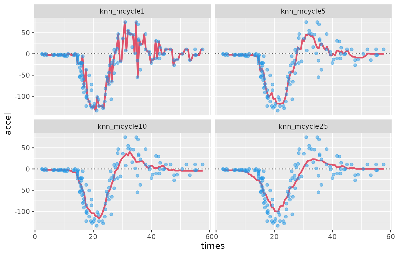

Plot methods for (multi-)model and “cv”:

The methods plot.model(), plot.multimodel() and plot.cv() generate scatter plots (ggplots) of actual responses versus predictions. plot.model() uses (in-sample) predictions from a single model fit, while plot.cv() displays the out-of-sample predictions resulting from the cross-validation.

i <- 1  # 1-nearest neighbor
gridExtra::arrangeGrob(
  plot(subset(knn_mcycle, i)) + # fits the model and plots response vs. fitted
    ggtitle("plot.model: in-sample fit of 1-NN"), 
  plot(subset(cv_mcycle, i)) +  # plots response vs. cv-fits
    ggtitle("plot.cv: out-of-sample fit"), 
  nrow = 1) %>% plot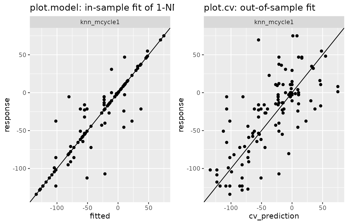

Plotting a multimodel or “cv” object including several models creates the same type of plot with one panel/facet for each model.

`tune()` a parameter

Starting from the `cv` object:

tune() is a generic function, and it method tune.cv() simply selects the best model according to test error, thus returning a “model” object:

tune(cv_mcycle)          # Selects the best model according to test error

## --- A "model" object ---
##   label:          knn_mcycle14
##   model class:    fm_knn
##   formula:        accel ~ times
##   data:           data.frame [133 x 2], input as: 'data = mcycle'
##   response_type:  continuous
##   call:           fm_knn(formula = accel ~ times, data = data, k = 14L)

tune(cv_mcycle) %>% fit  # Back to non-modeltuner world (fitted model)

## k-nearest neighbors model (class 'fm_knn')
##   formula:      accel ~ times - 1
##   data:         data
##   k:            14
##   n:            133
##   standardize:  TRUE
##   weighted:     FALSE

“Shortcut methods” `tune.model()` and `tune.default()`

tune.model() takes an object of class “model” and returns a “tuned” version.

mod_mcycle <- model(fm_mcycle)
mod_mcycle %>% tune(k = 1:25)   # "Dots" in tune(x, ...) are passed to multimodel()

## --- A "model" object ---
##   label:          model9
##   model class:    fm_knn
##   formula:        accel ~ times
##   data:           data.frame [133 x 2], input as: 'data = mcycle'
##   response_type:  continuous
##   call:           fm_knn(formula = accel ~ times, data = data, k = 9L)

The code line mod_mcycle %>% tune(k = 1:25) executes mod_mcycle %>% multimodel(k = 1:25) %>% cv %>% tune.

Likewise, tune.default() takes a fitted model and returns a fitted model (result not shown).

fm_mcycle %>% tune(k = 1:25)

This runs fm_mcycle %>% model %>% multimodel(k = 1:20) %>% cv %>% tune %>% fit

Binary response

We now fit a glm to the kyphosis data from package rpart:

library(rpart, warn.conflicts = FALSE)
data(kyphosis, package = "rpart")
head(kyphosis)

##   Kyphosis Age Number Start
## 1   absent  71      3     5
## 2   absent 158      3    14
## 3  present 128      4     5
## 4   absent   2      5     1
## 5   absent   1      4    15
## 6   absent   1      2    16

table(kyphosis$Kyphosis)

## 
##  absent present 
##      64      17

# glm model (fitted model)
glmmod <- glm(Kyphosis == "present" ~ ., kyphosis, family = "binomial")
summary(glmmod)

## 
## Call:
## glm(formula = Kyphosis == "present" ~ ., family = "binomial", 
##     data = kyphosis)
## 
## Coefficients:
##              Estimate Std. Error z value Pr(>|z|)   
## (Intercept) -2.036934   1.449575  -1.405  0.15996   
## Age          0.010930   0.006446   1.696  0.08996 . 
## Number       0.410601   0.224861   1.826  0.06785 . 
## Start       -0.206510   0.067699  -3.050  0.00229 **
## ---
## Signif. codes:  0 '***' 0.001 '**' 0.01 '*' 0.05 '.' 0.1 ' ' 1
## 
## (Dispersion parameter for binomial family taken to be 1)
## 
##     Null deviance: 83.234  on 80  degrees of freedom
## Residual deviance: 61.380  on 77  degrees of freedom
## AIC: 69.38
## 
## Number of Fisher Scoring iterations: 5

`model` object

In modeltuner, a binary response is expected to have values 0 and 1. If this is the case, the response_type will be “binary” (otherwise “continuous”), and cv_performance() will use the logLoss metric by default (in contrast to rmse for a continuous response). See ?metrics and ?default_metric for more information.

mod1_kyph <- model(glmmod, label = "glm")
mod1_kyph

## --- A "model" object ---
##   label:          glm
##   model class:    glm
##   formula:        Kyphosis == "present" ~ Age + Number + Start
##   data:           data.frame [81 x 4], input as: 'data = kyphosis'
##   response_type:  binary
##   call:           glm(formula = Kyphosis == "present" ~ ., family = "binomial", data = data)
##   fit:            Object of classes 'glm', 'lm'

Cross-validate and evaluate result

Below, mod1_kyph is cross-validated and the result is evaluated with the default metric and a standard metric.

cv_kyph <- cv(mod1_kyph)
cv_performance(cv_kyph)

## --- Performance table ---
## Metric: logLoss
##     train_logLoss test_logLoss time_cv
## glm       0.37571      0.44412   0.017

cv_performance(cv_kyph, metric = list(cl_err = classification_error))

## --- Performance table ---
## Metric: cl_err
##     train_cl_err test_cl_err time_cv
## glm      0.15638     0.22222   0.017

Plot of a model/multimodel/cv in case of binary response:

plot.model() and plot.cv() generate two separate violin plots of predicted values for the two groups of observations having response value 0 and 1:

# plot.(multi)model and plot.cv in binary case
gridExtra::arrangeGrob(
  plot(mod1_kyph) + ggtitle("plot.model: glm model"),
  plot(mod1_kyph %>% cv) + ggtitle("plot.cv: glm model"),
  nrow = 1) %>% plot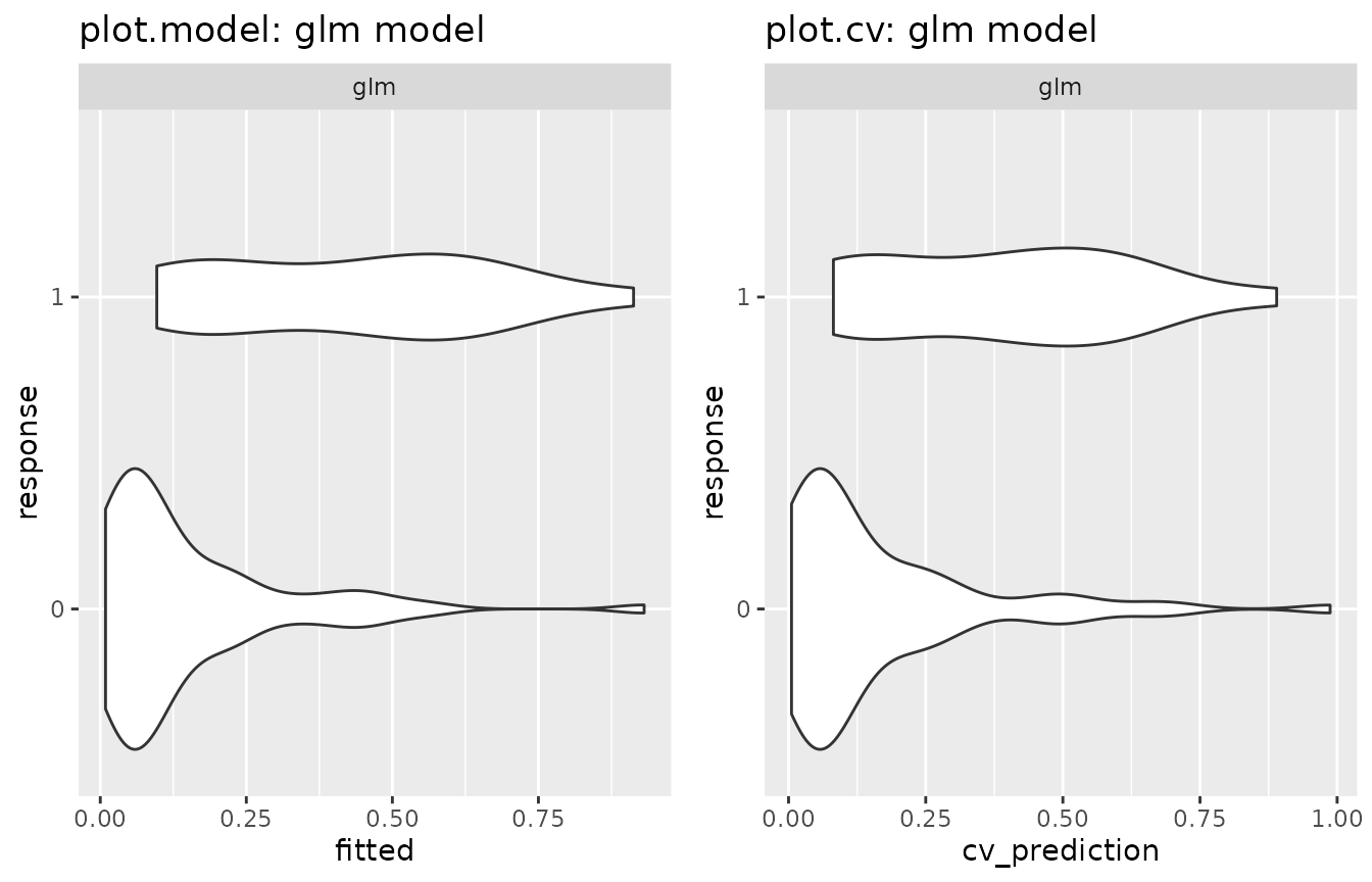

Alternative model: `ranger`

As an second model in the kyphosis example, ranger() is used to fit a random forest:

library(ranger)
# without fitting the model...
mod2_kyph <- model("ranger", Kyphosis == "present" ~ ., kyphosis, 
                   num.trees = 100, max.depth = 4, 
                   class = "ranger", label = "ranger")

The plot below shows that the random forest overfits the data in this example:

gridExtra::arrangeGrob(
  plot(mod2_kyph) + ggtitle("plot.model"),  # overfits
  plot(cv(mod2_kyph)) + ggtitle("plot.cv"),
  nrow = 1) %>% plot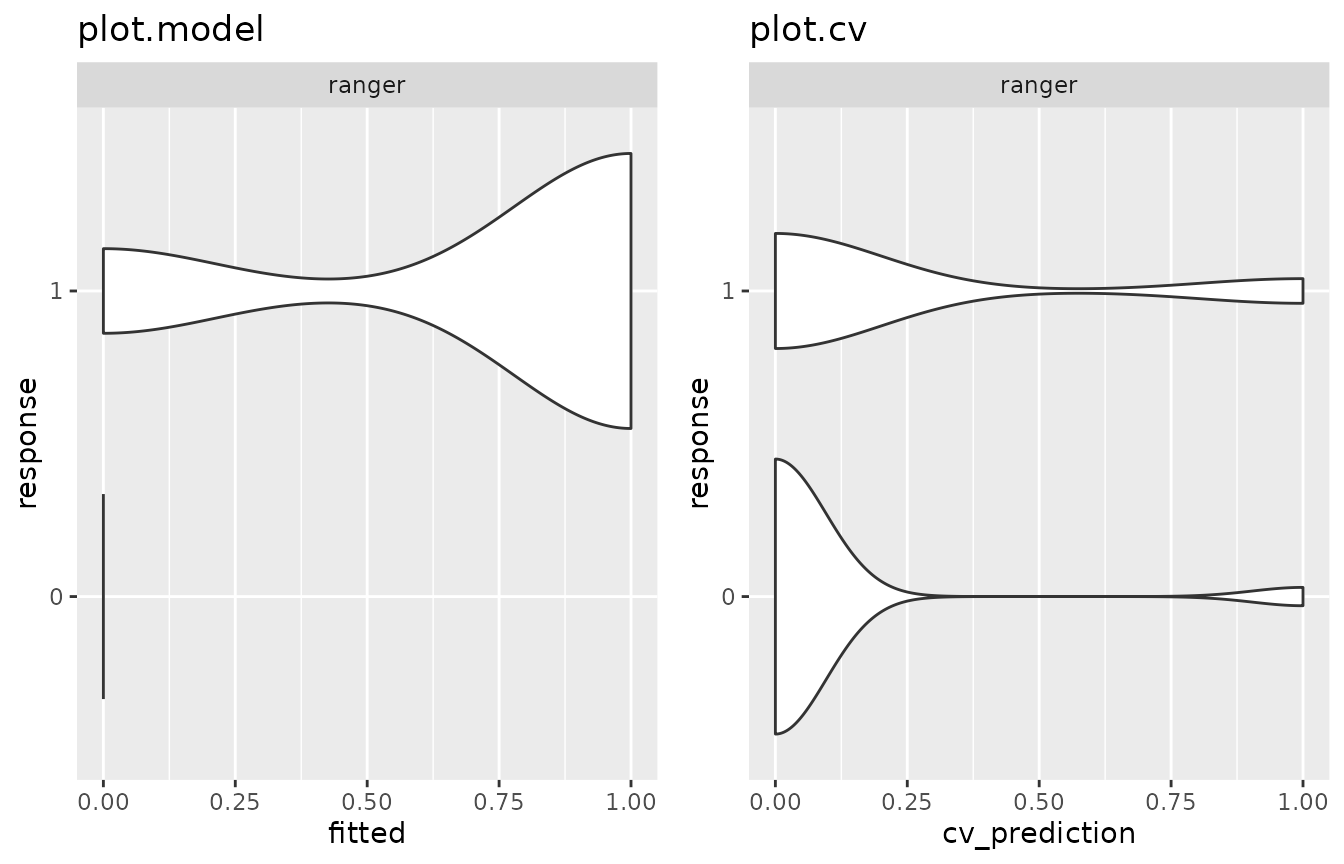

Combine the two models in a multimodel

# cv_performance
mm_kyph <- c(mod1_kyph, mod2_kyph)
cv_performance(mm_kyph)

## --- Performance table ---
## Metric: logLoss
##        train_logLoss test_logLoss time_cv
## glm          0.37465      0.46969   0.017
## ranger       2.46928      7.71019   0.048

Variable selection procedures based on cross-validation

The modeltuner package has a collection of functions that modify a given model by adding or removing variables from the formula and optionally cross-validate them.

For the sake of more compact formulas in printed output, we first introduce a variable transformation in kyphosis and redefine the model mod1_kyph:

mod1_kyph <- update(mod1_kyph, 
                    data = transform(kyphosis, 
                                     kyphosisFlag = Kyphosis == "present"), 
                    formula = kyphosisFlag ~ .)

Combine all models resulting from removing or adding one variable

step_reduce() includes all models resulting from removing one variable from the full model,
step_extend() includes all models resulting from adding one variable to base model.

The full model and base model are defined in the parameters formula1 and formula2. When formula1 and formula2 are not given by the user, the actual model is taken as the full model and a bare intercept model as the base model. See ?stepwise for more details. step_reduce() and step_extend() return a “cv” object if the argument cv is TRUE (the default) or a multimodel if cv=FALSE.

step_reduce(mod1_kyph, cv = FALSE)  # remove one variable from full model

## --- A "multimodel" object containing 3 models ---
## 
## '-Age':
##   model class:  glm
##   formula:      kyphosisFlag ~ Number + Start
##   data:         data.frame [81 x 5], 
##                 input as: 'data = transform(kyphosis, kyphosisFlag = Kyphosis == "present")'
##   call:         glm(formula = kyphosisFlag ~ Number + Start, family = "binomial", data = data)
## 
## '-Number':
##   model class:  glm
##   formula:      kyphosisFlag ~ Age + Start
##   data:         data.frame [81 x 5], 
##                 input as: 'data = transform(kyphosis, kyphosisFlag = Kyphosis == "present")'
##   call:         glm(formula = kyphosisFlag ~ Age + Start, family = "binomial", data = data)
## 
## '-Start':
##   model class:  glm
##   formula:      kyphosisFlag ~ Age + Number
##   data:         data.frame [81 x 5], 
##                 input as: 'data = transform(kyphosis, kyphosisFlag = Kyphosis == "present")'
##   call:         glm(formula = kyphosisFlag ~ Age + Number, family = "binomial", data = data)
## 
## Parameter table:
##                               formula
## -Age    kyphosisFlag ~ Number + Start
## -Number kyphosisFlag ~ Age + Start   
## -Start  kyphosisFlag ~ Age + Number

step_extend(mod1_kyph, cv = FALSE)  # add one variable to base model

## --- A "multimodel" object containing 3 models ---
## 
## '+Age':
##   model class:  glm
##   formula:      kyphosisFlag ~ Age
##   data:         data.frame [81 x 5], 
##                 input as: 'data = transform(kyphosis, kyphosisFlag = Kyphosis == "present")'
##   call:         glm(formula = kyphosisFlag ~ Age, family = "binomial", data = data)
## 
## '+Number':
##   model class:  glm
##   formula:      kyphosisFlag ~ Number
##   data:         data.frame [81 x 5], 
##                 input as: 'data = transform(kyphosis, kyphosisFlag = Kyphosis == "present")'
##   call:         glm(formula = kyphosisFlag ~ Number, family = "binomial", data = data)
## 
## '+Start':
##   model class:  glm
##   formula:      kyphosisFlag ~ Start
##   data:         data.frame [81 x 5], 
##                 input as: 'data = transform(kyphosis, kyphosisFlag = Kyphosis == "present")'
##   call:         glm(formula = kyphosisFlag ~ Start, family = "binomial", data = data)
## 
## Parameter table:
##                       formula
## +Age    kyphosisFlag ~ Age   
## +Number kyphosisFlag ~ Number
## +Start  kyphosisFlag ~ Start

Backward elimination and forward selection

step_forward() applies step_extend() repeatedly, selecting the best model w.r.t. test error at each step, thus performing a forward selection of variables.
step_backward() applies step_reduce() repeatedly, selecting the best model w.r.t. test error at each step, thus performing a backward elimination of variables.

Backward elimination:

(backwd <- step_backward(mod1_kyph))

## --- A "cv" object containing 4 validated models ---
## 
## Validation procedure: Complete k-fold Cross-Validation
##   Number of obs in data:   81
##   Number of test sets:     10
##   Size of test sets:       ~8
##   Size of training sets:  ~73
## 
## Models:
## 
## 'full':
##   model class:  glm
##   formula:      kyphosisFlag ~ Age + Number + Start
##   metric:       logLoss
## 
## '-Number':
##   model class:  glm
##   formula:      kyphosisFlag ~ Age + Start
##   metric:       logLoss
## 
## '-Age':
##   model class:  glm
##   formula:      kyphosisFlag ~ Start
##   metric:       logLoss
## 
## and 1 model more, labelled:
##   '-Start'
## 
## 
## Parameter table:
##                                     formula
## full    kyphosisFlag ~ Age + Number + Start
## -Number kyphosisFlag ~ Age + Start         
## -Age    kyphosisFlag ~ Start               
## -Start  kyphosisFlag ~ 1

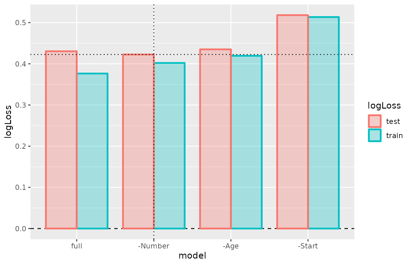
cv_performance(backwd)

## --- Performance table ---
## Metric: logLoss
##                                     formula train_logLoss test_logLoss time_cv
## full    kyphosisFlag ~ Age + Number + Start       0.37638      0.43046   0.017
## -Number kyphosisFlag ~ Age + Start                0.40207      0.42260   0.014
## -Age    kyphosisFlag ~ Start                      0.41942      0.43510   0.013
## -Start  kyphosisFlag ~ 1                          0.51356      0.51815   0.012

Plot the performance table of backwd:

backwd %>% cv_performance %>% plot

Forward selection:

forwd <- step_forward(mod1_kyph)

Best subset model selection

best_subset() combines submodels of the full model in a multimodel and subjects it to cv(). The desired range of the model sizes (number of regressors) to include is specified in the parameter nvars. best_subset() returns either a “cv” object (if cv=TRUE, default) or a multimodel, depending on parameter cv.

# best subset selection
(bestsub <- best_subset(mod1_kyph, nvars = 1:2))

## --- A "cv" object containing 6 validated models ---
## 
## Validation procedure: Complete k-fold Cross-Validation
##   Number of obs in data:   81
##   Number of test sets:     10
##   Size of test sets:       ~8
##   Size of training sets:  ~73
## 
## Models:
## 
## '+Age':
##   model class:  glm
##   formula:      kyphosisFlag ~ Age
##   metric:       logLoss
## 
## '+Number':
##   model class:  glm
##   formula:      kyphosisFlag ~ Number
##   metric:       logLoss
## 
## '+Start':
##   model class:  glm
##   formula:      kyphosisFlag ~ Start
##   metric:       logLoss
## 
## and 3 models more, labelled:
##   '+Age+Number', '+Age+Start', '+Number+Start'
## 
## 
## Parameter table:
##                                     formula
## +Age          kyphosisFlag ~ Age           
## +Number       kyphosisFlag ~ Number        
## +Start        kyphosisFlag ~ Start         
## ... 3 rows omitted (nrow=6)

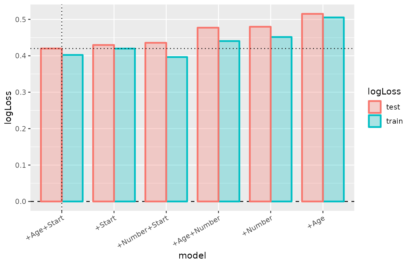
bestsub %>% 
  cv_performance %>%
  sort_models(by = "test") %>%   # sort models by test error
  plot +
  theme(axis.text.x = element_text(angle = 30, vjust = 1, hjust=1))

Mathias Ambuehl

2023-12-28

Basics

The formula interface

Fitted models and objects of class “model”

Cross validation

Folds

Execute a cross-validation: `cv()`

Evaluate a cross-validation: `cv_performance()`

Saving the model fits

Multimodels

Cross-validate a multimodel

Find the best-fitting model: `tune()`

Number of models and model labels: `n_model()`, `label()`

Subsetting a multimodel or “cv” object with `subset()`

Extraction of a model from a multimodel or “cv” object: `extract_model()`

Sort the models: `sort_models()`

Hyperparameter tuning

Motivating example: Parameter `k` in k-nearest-neighbor

Create a multimodel with `multimodel()`

Plot a performance table

Plot methods for (multi-)model and “cv”:

`tune()` a parameter

Starting from the `cv` object:

“Shortcut methods” `tune.model()` and `tune.default()`

Binary response

`model` object

Cross-validate and evaluate result

Plot of a model/multimodel/cv in case of binary response:

Alternative model: `ranger`

Combine the two models in a multimodel

Variable selection procedures based on cross-validation

Combine all models resulting from removing or adding one variable

Backward elimination and forward selection

Best subset model selection

An introduction to modeltuner with examples

Mathias Ambuehl

2023-12-28

Basics

The formula interface

Fitted models and objects of class “model”

Cross validation

Folds

Execute a cross-validation: cv()

Evaluate a cross-validation: cv_performance()

Saving the model fits

Multimodels

Cross-validate a multimodel

Find the best-fitting model: tune()

Manipulation of multimodels and related objects

Number of models and model labels: n_model(), label()

Subsetting a multimodel or “cv” object with subset()

Extraction of a model from a multimodel or “cv” object: extract_model()

Sort the models: sort_models()

Hyperparameter tuning

Motivating example: Parameter k in k-nearest-neighbor

Create a multimodel with multimodel()

Plot a performance table

Plot methods for (multi-)model and “cv”:

tune() a parameter

Starting from the cv object:

“Shortcut methods” tune.model() and tune.default()

Binary response

model object

Cross-validate and evaluate result

Plot of a model/multimodel/cv in case of binary response:

Alternative model: ranger

Combine the two models in a multimodel

Variable selection procedures based on cross-validation

Combine all models resulting from removing or adding one variable

Backward elimination and forward selection

Best subset model selection

Execute a cross-validation: `cv()`

Evaluate a cross-validation: `cv_performance()`

Find the best-fitting model: `tune()`

Number of models and model labels: `n_model()`, `label()`

Subsetting a multimodel or “cv” object with `subset()`

Extraction of a model from a multimodel or “cv” object: `extract_model()`

Sort the models: `sort_models()`

Motivating example: Parameter `k` in k-nearest-neighbor

Create a multimodel with `multimodel()`

`tune()` a parameter

Starting from the `cv` object:

“Shortcut methods” `tune.model()` and `tune.default()`

`model` object

Alternative model: `ranger`