Fitting and tuning Iteratively Fitted Models

Iteratively Fitted Models

Introductory remark: In this vignette, it is assumed that the reader is familiar with the main concepts of the modeltuner package, in particular the classes “model”, “multimodel”, “cv” and the related functions and methods. If this is not the case, reading the introductory vignette “An introduction to modeltuner with examples” (vignette(modeltuner)) first is recommended.

We speak of an iteratively fitted model (IFM) when the output of the model fitting function is not just a single model, but rather a sequence of models of increasing structural complexity. Examples are gradient boosting (as implemented in package xgboost) or Lasso regression and elastic nets (available from package glmnet).

Such a sequence of models begins with a simple model (often a constant model) and ends with a model that possibly seriously overfits the training data. Within the sequence, training error typically decreases successively, while test error decreases in early iterations, then at some point stagnates or starts increasing again.

We use the term iterations to refer to element models in the sequence, although properly speaking, the actual fitting process does not need be iterative. In the two cases mentioned above, gradient boosting and regularized linear models, the fitting process actually is iterative. In the analysis tools to be introduced in this vignette, the availability of predictions for each iteration is crucial, such that training and test error can be computed for each iteration.

The bias-variance trade-off

When working with IFMs, one of the the key tasks consists in finding an appropriate iteration or model, one that is not too simple and at the same time does not excessively (over)fit the training data. In short, we strive for a good compromise in a situation of bias-variance trade-off. While a simple model suffers from bias, a model that approximates the training data too closely has the disadvantage of a large variance.

Boosted trees: `fm_xgb()`

A single model

This example uses simulated data generated by the function simuldat(), included in modeltuner.

library(modeltuner)
options(cv_verbose = FALSE, width = 100) 
library(magrittr, warn.conflicts = FALSE)   # for pipe operator

# Simulated data set
set.seed(123)
d <- simuldat()

We can define an xgboost model in terms of formula and data with the function fm_xgb():

fm0 <- fm_xgb(Y ~ ., d)
fm0

## Fitted model of class 'fm_xgb' 
##   formula:     Y ~ X1 + X2 + X3 + X4 + X5 + X6 + X7 + X8 + X9 + X10 + g - 1
##   data:        d (500 rows)
##   call:        fm_xgb(formula = Y ~ ., data = d)
##   nfeatures:   30
##   iterations:  100
##   pref_iter:   100

model() creates an object of class “model”:

# Model
m0 <- model(fm0, label = "xgb")

Evaluation log of a model

A model’s evaluation_log() consists in the sequence of training errors, but does not provide any indication as to where a good balance between oversimplifying and overfitting is to be found.

# evaluation log of an object of class "model"
evaluation_log(m0)

## 'evaluation_log', 1 model:
## 
## Model 'xgb':
##   model class: fm_xgb
##  iter train_rmse test_rmse
##     1     3.5772        NA
##    21     0.3939        NA
##    41     0.1484        NA
##    60     0.0671        NA
##    80     0.0268        NA
##   100     0.0123        NA

plot(evaluation_log(m0))

## Warning: Removed 100 rows containing missing values (`geom_point()`).

## Warning: Removed 100 rows containing missing values (`geom_line()`).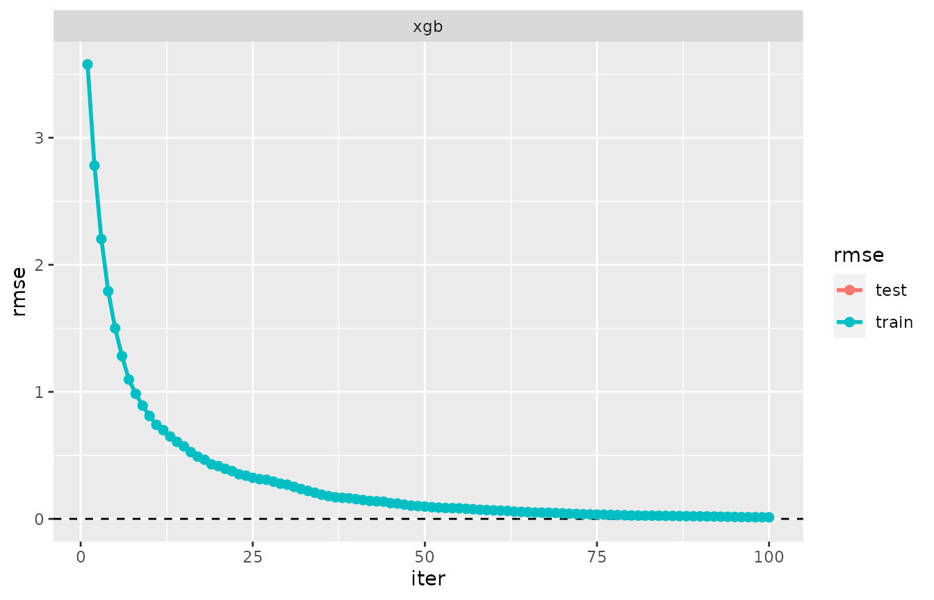

Note that we could also have applied evaluation_log() to the fitted model fm0.

Cross-validation

Running a cross validation with cv() yields a cross-validated model, of class “cv”. The evaluation log now includes both training and test error.

# evaluation log of an object of class "cv"
cvm <- cv(m0)
evaluation_log(cvm)

## 'evaluation_log', 1 cross-validated model:
## 
## Model 'xgb':
##   model class: fm_xgb
##  iter train_rmse test_rmse criterion
##     1     3.5736      3.77          
##    15     0.5281      2.11          
##    30     0.2326      2.05          
##    44     0.1239      2.03          
##    59     0.0650      2.03          
##    63     0.0542      2.03       min
##    73     0.0361      2.03

plot(evaluation_log(cvm))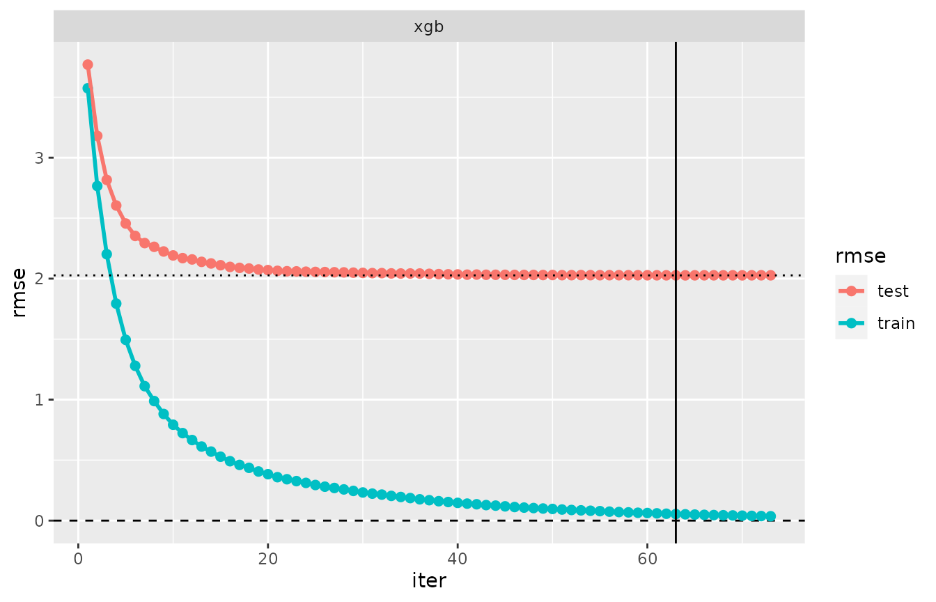

In this plot, the vertical line marks the iteration having minimal test error. By default, this iteration is considered the preferred one. In the example, iteration 63 is preferred. cv_performance() returns training and test error recorded at this iteration:

cv_performance(cvm)

## --- Performance table ---
## Metric: rmse
##     train_rmse test_rmse iteration time_cv
## xgb   0.054174    2.0271        63    0.71

Back to model and fitted model

If we now take a step back, extracting the model object from cvm, the information on the best (preferred) iteration is attached to the resulting model object:

# back to model
m1 <- extract_model(cvm) # or: tune(cvm)
m1

## --- A "model" object ---
##   label:          xgb
##   model class:    fm_xgb
##   formula:        Y ~ X1 + X2 + X3 + X4 + X5 + X6 + X7 + X8 + X9 + X10 + g - 1
##   data:           data.frame [500 x 12], input as: 'data = d'
##   response_type:  continuous
##   call:           fm_xgb(formula = Y ~ ., data = data)
##   fit:            Object of class 'fm_xgb'
## Preferred iteration from cv:  iter=63

In the final line of the output above, the best iteration according to cross-validation results is reported. Apart from that, m1 is identical with the original model object m0.

Finally, on fitting this model, thus converting a “model” object to a fitted model, the nrounds argument is adjusted according to the preference resulting from cross-validation:

# back to fitted model
fm1 <- fit(m1)

## set_pref_iter(), model 'xgb', modifications made in call:
##   pref_iter=63, nrounds=63, early_stopping_rounds=NULL

getCall(fm1)

## fm_xgb(formula = Y ~ ., data = d, nrounds = 63L, pref_iter = 63L, 
##     early_stopping_rounds = NULL)

Note that the number of rounds has been fixed to nrounds=63 in the fitting call.

Tuning `nrounds` with `tune()`

Applying tune() to a IFM without further arguments triggers a cross-validation and returns the adjusted model (model or fitted) with “tuned” number of rounds:

tune(m0)  # executes m0 %>% cv %>% extract_model
tune(fm0) # executes fm0 %>% model %>% cv %>% extract_model %>% fit

Repeated executions will result in varying choices of nrounds, as new cross-validation groups (folds) are randomly generated at each execution, leading to different a evaluation log.

Default metric for xgboost models

“cv” objects based on a model created with fm_xgb() differ from any other model class in the way how their metric is selected by default. They currently are the only model type not having the standard choice, which is rmse for continuous response and logLoss in the binary case.

Each xgboost model has an eval_metric. If not specified explicitly by the user, this metric is set depending on the argument objective in the call to xgb.train() or fm_xgb(). For example, objective="reg:linear" has rmse as its default eval_metric, while objective="binary:logistic" chooses logloss. In modeltuner, the eval_metric is taken as the default metric of the resulting “cv” object.

As an example, consider a model using the eval_metric “mphe” (mean pseudo-Huber error). This is the default eval_metric for objective="reg:pseudohubererror".

data(diamonds, package = "ggplot2")
set.seed(1)
diamonds <- diamonds[sample(nrow(diamonds), 5000), ]
xgb_phe <- model(fm_xgb(log(price) ~ . , diamonds, objective = "reg:pseudohubererror"),
                 base_score = median(log(diamonds$price)),
            label = "xgb_pseudohuber")
cv_phe <- cv(xgb_phe)
cv_performance(cv_phe)

## --- Performance table ---
## Metric: mphe
##                 train_mphe test_mphe iteration time_cv
## xgb_pseudohuber  0.0010635 0.0062366        99    3.13

The values of the metric “mphe” (and the evaluation log) are read from the return value of xgb.train() or xgb.cv() - we actually don’t necessarily need an R function mphe() evaluating this metric in the modeltuner implementation.

cv_performance() can still be executed with any available metric:

cv_performance(cv_phe, metric = "mae")

## --- Performance table ---
## Metric: mae
##                 train_mae test_mae iteration time_cv
## xgb_pseudohuber  0.033856 0.081742        99    3.13

In case of doubt on the default metric of a model, one may use the function default_metric(). It identifies the metric function that will be used by default:

default_metric(xgb_phe)  # no metric function, only a name (values read from xgboost output)

## $mphe
## NULL

default_metric(m1)       # metric available, only its name

## $rmse
## function (actual, predicted, w = NULL, ...) 
## {
##     sqrt(mse(actual = actual, predicted = predicted, w = w, ...))
## }
## <bytecode: 0x55b4c8185d58>
## <environment: namespace:MetricsWeighted>

Hyperparameter tuning

In this section, we investigate the effect of modifying the value of parameter max_depth in model m0. A multimodel is defined by expanding max_depth from 1 to 6:

# Generate a multimodel
mm_depth <- multimodel(m0, prefix = "xgb_depth", max_depth = 1:6, 
                       nrounds = 200)

Cross-validation

cv() runs separate cross-validations for the 6 models, using identical folds for all of them.

cvmm_depth <- cv(mm_depth)
cvmm_depth

## --- A "cv" object containing 6 validated models ---
## 
## Validation procedure: Complete k-fold Cross-Validation
##   Number of obs in data:  500
##   Number of test sets:     10
##   Size of test sets:       50
##   Size of training sets:  450
## 
## Models:
## 
## 'xgb_depth1':
##   model class:  fm_xgb
##   formula:      Y ~ X1 + X2 + X3 + X4 + X5 + X6 + X7 + X8 + X9 + X10 + g
##   metric:       rmse
## 
## 'xgb_depth2':
##   model class:  fm_xgb
##   formula:      Y ~ X1 + X2 + X3 + X4 + X5 + X6 + X7 + X8 + X9 + X10 + g
##   metric:       rmse
## 
## 'xgb_depth3':
##   model class:  fm_xgb
##   formula:      Y ~ X1 + X2 + X3 + X4 + X5 + X6 + X7 + X8 + X9 + X10 + g
##   metric:       rmse
## 
## and 3 models more, labelled:
##   'xgb_depth4', 'xgb_depth5', 'xgb_depth6'
## 
## 
## Parameter table:
##            max_depth nrounds
## xgb_depth1         1     200
## xgb_depth2         2     200
## xgb_depth3         3     200
## ... 3 rows omitted (nrow=6)
## 
## Preferred iterations:
##   model 'xgb_depth1':  min (iter=144)
##   model 'xgb_depth2':  min (iter=151)
##   model 'xgb_depth3':  min (iter=91)
## ... and 3 lines more.

The printed output lists details for the first 3 models only by default. In order to get display details on all 6 models output, we could use the argument n in print() (output not shown):

print(cvmm_depth, n = 6)

The function extract_pref_iter() extracts the preferred iterations from a “cv” object:

extract_pref_iter(cvmm_depth)

## Preferred iterations:
##   model 'xgb_depth1':  min (iter=144)
##   model 'xgb_depth2':  min (iter=151)
##   model 'xgb_depth3':  min (iter=91)
##   model 'xgb_depth4':  min (iter=117)
##   model 'xgb_depth5':  min (iter=99)
##   model 'xgb_depth6':  min (iter=67)

`cv_performance()` and `evaluation_log()`

The output of these functions (be it printed or plotted) extends what we have seen for a single model above to the multiple model case:

plot(cv_performance(cvmm_depth))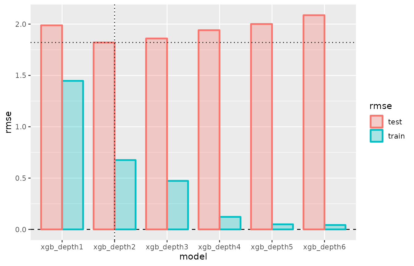

plot(evaluation_log(cvmm_depth))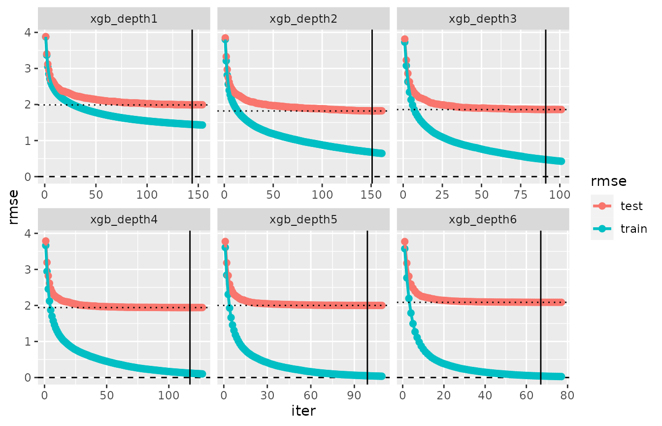

The plot of the performance table can be enhanced by setting xvar=max_depth:

plot(cv_performance(cvmm_depth), xvar = "max_depth")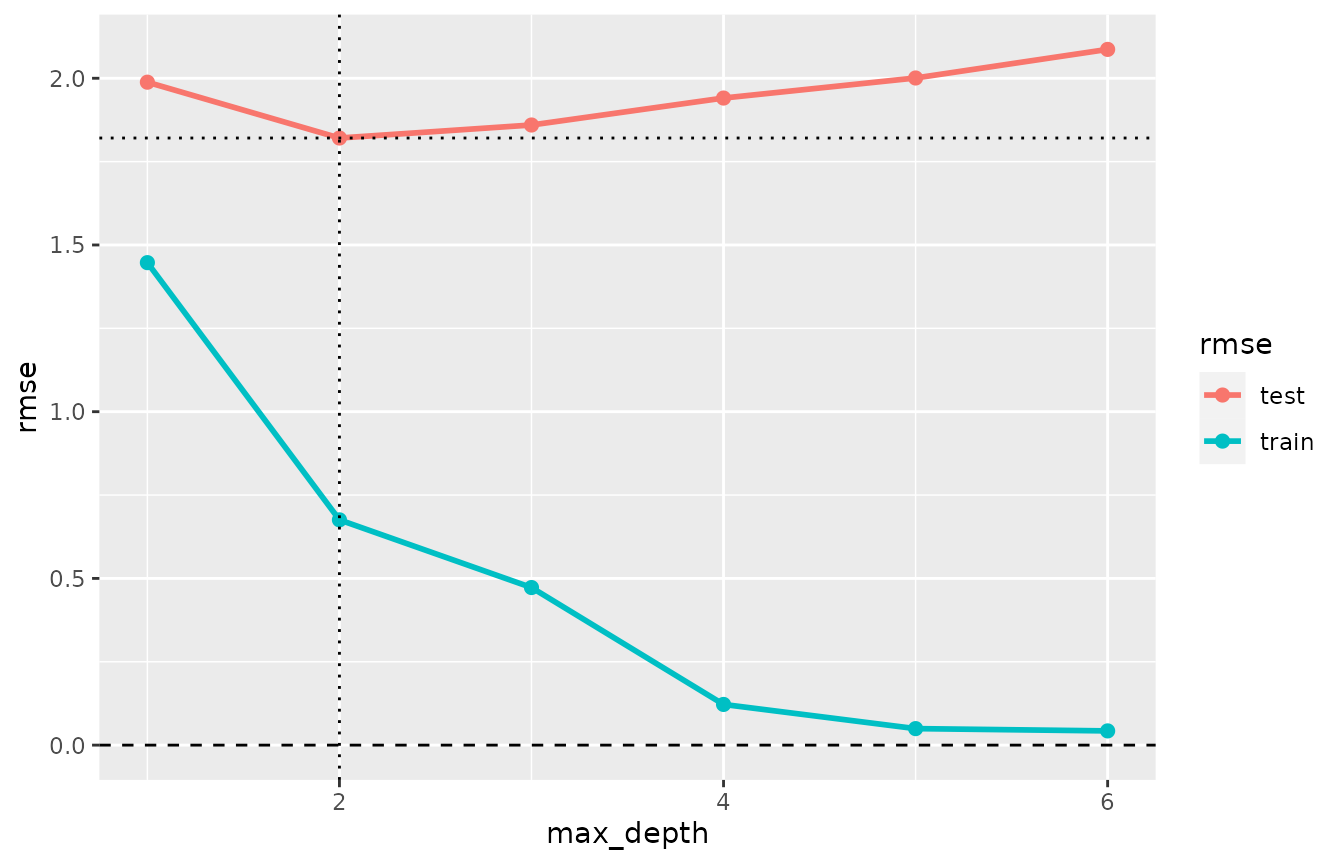

The plot shows how values max_depth>2 do not improve the predictive performance on unseen data, but increasingly overfit the training data.

Tuning and extracting a model or fitted model from a “cv” object

Applying tune() to cvmm_depth will pick the best-performing model (that having lowest test error) and return it.

m_tuned <- tune(cvmm_depth)
fm_tuned <- fit(m_tuned)

## set_pref_iter(), model 'xgb_depth2', modifications made in call:
##   pref_iter=151, nrounds=151, early_stopping_rounds=NULL

getCall(fm_tuned)

## fm_xgb(formula = Y ~ X1 + X2 + X3 + X4 + X5 + X6 + X7 + X8 + 
##     X9 + X10 + g, data = data, nrounds = 151L, early_stopping_rounds = NULL, 
##     pref_iter = 151L, max_depth = 2L)

Preference criteria for iterations

Basics on preference criteria

So far, it has been assumed throughout that the preferred model is the one having minimal test error. Depending on the current application and its goals, other choices may be desirable. For example, some users may want stable models in the sense that they expect that fitting the model with different data sets yields results that differ no too much. In the example of multimodel mm above, the model with max_depth=2 has the lowest test error, but still the analyst may favor choosing max_depth=1, as it exhibits less overfitting.

modeltuner offers various alternative preference/selection criteria. The default criterion, used in all examples so far, was

crit_min()

## Preference criterion for an iteratively fitted model:
##   criterion:     crit_min()
##   label suffix:  "min"
##   Selects the iteration with minimal test error.

To choose a criterion, you use the argument iter in cv(). The call cv(mm) could also be written as

cvm <- cv(m0, iter = crit_min()) # same as: cvm <- cv(m0)

Alternative criteria

Two criteria that avoid selecting a too heavily overfitting model are crit_se() and crit_overfit(). They are explained in the printed output below:

crit_se(factor = 2)         # default: factor=1

## Preference criterion for an iteratively fitted model:
##   criterion:     crit_se(2)
##   label suffix:  "2se"
##   Selects the first iteration where test error does not exceed
##     the minimal test error by more than 2 standard errors.

crit_overfit(ratio = 0.8)  # default: ratio=0.9

## Preference criterion for an iteratively fitted model:
##   criterion:     crit_overfit(0.8)
##   label suffix:  "overfit0.8"
##   Selects the iteration with minimal test error among those where
##   the ratio of training and test error does not fall below 0.8.

More available criteria are

crit_first()
crit_last()
crit_iter(20) # fixed iteration number

Specifying a criterion in `cv()`

We now cross-validate the model m0 again, thereby claiming that the ratio of training and test error remains above 0.75. We do this by choosing the criterion iter = crit_overfit(0.75), thus ensuring that predictive performances are compared between models sharing a similar degree of overfitting.

# cv()
cvm_ovf075 <- cv(m0, iter = crit_overfit(0.75))
cvm_ovf075

## --- A "cv" object containing 1 validated model ---
## 
## Validation procedure: Complete k-fold Cross-Validation
##   Number of obs in data:  500
##   Number of test sets:     10
##   Size of test sets:       50
##   Size of training sets:  450
## 
## Model:
## 
## 'xgb':
##   model class:  fm_xgb
##   formula:      Y ~ X1 + X2 + X3 + X4 + X5 + X6 + X7 + X8 + X9 + X10 + g - 1
##   metric:       rmse
## 
## Preferred iterations:
##   model 'xgb':  overfit0.75 (iter=3)

plot(evaluation_log(cvm_ovf075))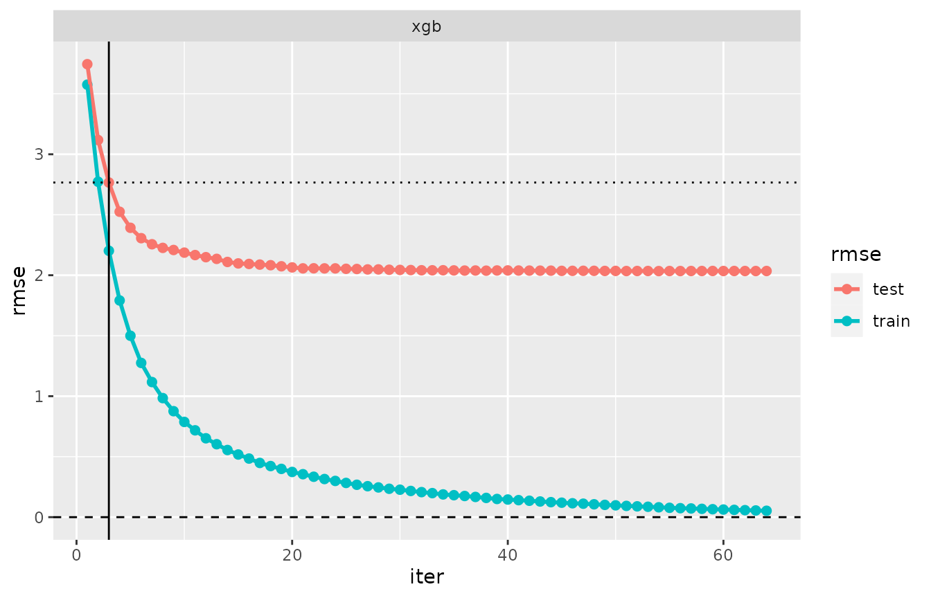

As a consequence of the different choice of a preference criterion, an earlier iteration (iteration 3) is selected than in cvm1 above with the default iter = crit_min(), where iteration 63 was preferred.

Back to model and fitted model

The preferred iteration is transformed back to a model and fitted model exactly as shown before in the crit_min() case:

m_tuned_ovf075 <- extract_model(cvm_ovf075)
fm_tuned_ovf075 <- fit(m_tuned_ovf075)

## set_pref_iter(), model 'xgb', modifications made in call:
##   pref_iter=3, nrounds=3, early_stopping_rounds=NULL

getCall(fm_tuned_ovf075)

## fm_xgb(formula = Y ~ ., data = d, nrounds = 3L, pref_iter = 3L, 
##     early_stopping_rounds = NULL)

Multimodel case

It is now straightforward to repeat the tuning of xgboost’s hyperparameter max_step with preference iter = crit_overfit(0.75).

cvmm_ovf075 <- cv(mm_depth, iter = crit_overfit(0.75))
extract_pref_iter(cvmm_ovf075)

## Preferred iterations:
##   model 'xgb_depth1':  overfit0.75 (iter=112)
##   model 'xgb_depth2':  overfit0.75 (iter=20)
##   model 'xgb_depth3':  overfit0.75 (iter=9)
##   model 'xgb_depth4':  overfit0.75 (iter=5)
##   model 'xgb_depth5':  overfit0.75 (iter=3)
##   model 'xgb_depth6':  overfit0.75 (iter=3)

plot(cv_performance(cvmm_ovf075), xvar = "max_depth")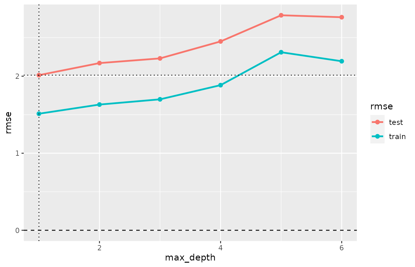

plot(evaluation_log(cvmm_ovf075)) + ggplot2::theme(legend.position = "bottom")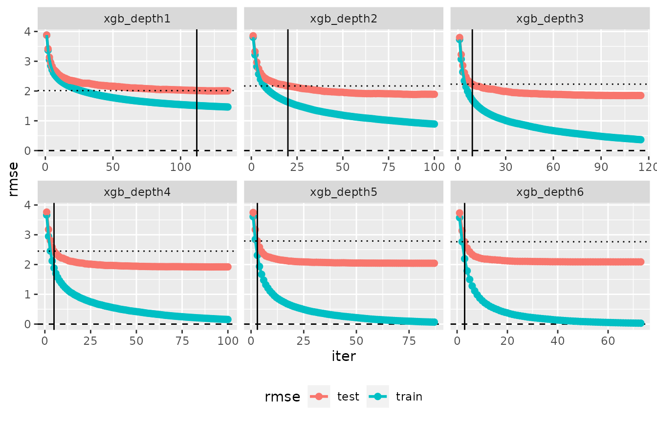

In contrast to hyperparameter tuning based on crit_min(), where max_depth=2 turned out to be the choice, tune(cvmm_ovf075) picks max_depth=1, which reflects the stronger reluctance to complex and more overfitting models expressed in iter=crit_overfit(0.75):

tune(cvmm_ovf075)

## --- A "model" object ---
##   label:          xgb_depth1
##   model class:    fm_xgb
##   formula:        Y ~ X1 + X2 + X3 + X4 + X5 + X6 + X7 + X8 + X9 + X10 + g
##   data:           data.frame [500 x 12], input as: 'data = d'
##   response_type:  continuous
##   call:           fm_xgb(formula = Y ~ ., data = data, nrounds = 200, max_depth = 1L)
## Preferred iteration from cv:  iter=112

Multiple preference criteria

cv() accepts multiple preference criteria. You just enclose the list of criteria in crit_list(...) or in c(...). The example below uses a model with maximal tree depth 2, and three preference criteria are given.

m_depth2 <- update(m0, nround = 200, max_depth = 2, label = "xgb_depth2")
cvm_depth2 <- cv(m_depth2, iter = c(crit_min(), crit_overfit(.7), crit_last()))
cvm_depth2

## --- A "cv" object containing 1 validated model ---
## 
## Validation procedure: Complete k-fold Cross-Validation
##   Number of obs in data:  500
##   Number of test sets:     10
##   Size of test sets:       50
##   Size of training sets:  450
## 
## Model:
## 
## 'xgb_depth2':
##   model class:  fm_xgb
##   formula:      Y ~ X1 + X2 + X3 + X4 + X5 + X6 + X7 + X8 + X9 + X10 + g
##   metric:       rmse
## 
## Preferred iterations:
##   model 'xgb_depth2':  min (iter=100), overfit0.7 (iter=28), last (iter=110)

plot(evaluation_log(cvm_depth2))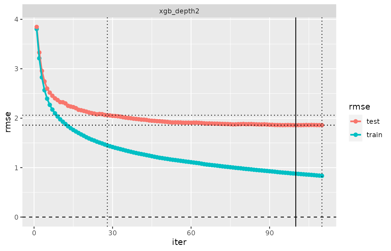

The cross-validated model cvm_depth2 includes three preference criteria. Let’s call the first of them the primary criterion. In the picture of the evaluation_log above, the iteration corresponding to the primary criterion is shown with a solid line, while all other criteria have a dotted line. In the printed output of an evaluation log, the primary criterion is marked with an asterisk:

evaluation_log(cvm_depth2)

## 'evaluation_log', 1 cross-validated model:
## 
## Model 'xgb_depth2':
##   model class: fm_xgb
##  iter train_rmse test_rmse  criterion
##     1      3.805      3.85           
##    23      1.548      2.09           
##    28      1.449      2.06 overfit0.7
##    45      1.231      1.95           
##    66      1.063      1.89           
##    88      0.937      1.88           
##   100      0.878      1.86 min*      
##   110      0.834      1.86 last

The role of the primary criterion is that cv_performance() returns training and test error from that iteration. The same is true for related functions, such as cv_predict() or plot.cv().

# cv_performance
cv_performance(cvm_depth2)

## --- Performance table ---
## Metric: rmse
##            train_rmse test_rmse iteration time_cv
## xgb_depth2    0.87816    1.8584       100   0.449

Changing the primary criterion: `set_pref_iter()`

The primary preference criterion of a “cv” object can be changed with the function set_pref_iter().

cvm_depth2_modif1 <- set_pref_iter(cvm_depth2, iter = crit_overfit(0.7))
plot(evaluation_log(cvm_depth2_modif1))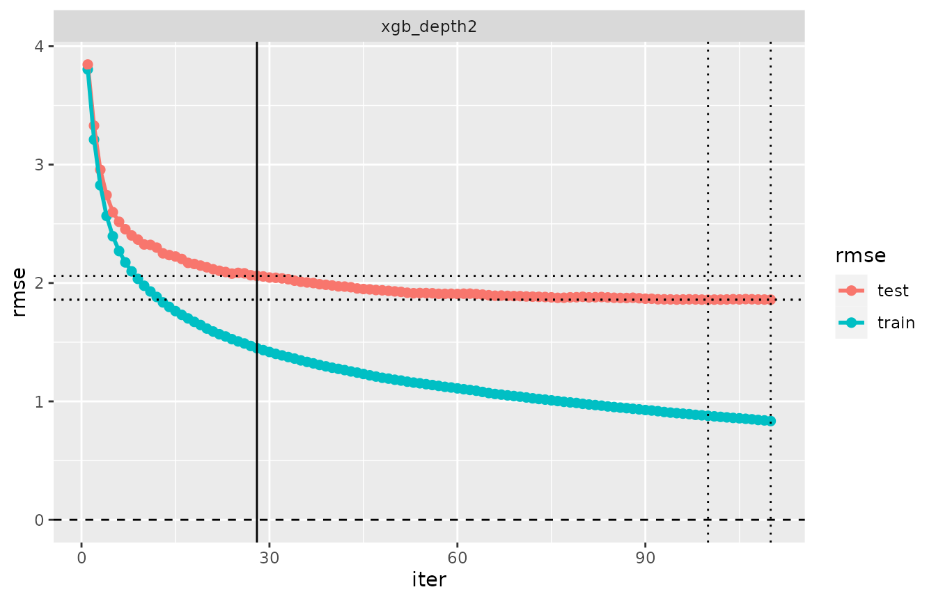

extract_pref_iter(cvm_depth2_modif1)

## Preferred iterations:
##   model 'xgb_depth2':  overfit0.7 (iter=28), min (iter=100), last (iter=110)

cv_performance(cvm_depth2_modif1)

## --- Performance table ---
## Metric: rmse
##            train_rmse test_rmse iteration time_cv
## xgb_depth2     1.4493    2.0601        28   0.449

# cv_performance() with different metric:
cv_performance(cvm_depth2_modif1, metric = "medae")

## --- Performance table ---
## Metric: medae
##            train_medae test_medae iteration time_cv
## xgb_depth2     0.95277     1.3459        28   0.449

set_pref_iter() is most useful when you specify a criterion that has previously been included in the cross-validation. If a criterion is chosen, some results will not be available:

# set_pref_iter with criteria not stated before in cv(..., iter = )
cvm_depth2_modif2 <- set_pref_iter(cvm_depth2, crit_iter(50))
cv_performance(cvm_depth2_modif2)  # available

## --- Performance table ---
## Metric: rmse
##            train_rmse test_rmse iteration time_cv
## xgb_depth2      1.183    1.9289        50   0.449

# cv_performance() with different metric:
cv_performance(cvm_depth2_modif2, metric = "medae") # required predictions are not available

## --- Performance table ---
## Metric: medae
##            train_medae test_medae iteration time_cv
## xgb_depth2          NA         NA        50   0.449

Note the difference: cv_performance() with the non-default metric="medae" is available for cvm_depth2_modif1 but not for cvm_depth2_modif2. The reason is that cross-validation predictions for iterations selected in the original “cv” object cvm_depth2 (i.e. for iterations 100, 28, 110) are stored in that object, but this is not the case for iteration 50. In order to obtain predictions for iteration 50, we need to re-run a cross validation, including crit_iter(50) in the list of criteria (or we could also set keep_fits=TRUE in cv() - see the section “Evaluation log for alternative metric” below).

`expand_pref_iter()`

Next, we introduce the function expand_pref_iter(), which converts a “cv” object with a single cross-validated model and multiple criteria to a “cv” object having several (essentially identical) models, but different preference criteria.

cvm_depth2_modif3 <- expand_pref_iter(cvm_depth2)
cvm_depth2_modif3

## --- A "cv" object containing 3 validated models ---
## 
## Validation procedure: Complete k-fold Cross-Validation
##   Number of obs in data:  500
##   Number of test sets:     10
##   Size of test sets:       50
##   Size of training sets:  450
## 
## Models:
## 
## 'xgb_depth2_min':
##   model class:  fm_xgb
##   formula:      Y ~ X1 + X2 + X3 + X4 + X5 + X6 + X7 + X8 + X9 + X10 + g
##   metric:       rmse
## 
## 'xgb_depth2_overfit0.7':
##   model class:  fm_xgb
##   formula:      Y ~ X1 + X2 + X3 + X4 + X5 + X6 + X7 + X8 + X9 + X10 + g
##   metric:       rmse
## 
## 'xgb_depth2_last':
##   model class:  fm_xgb
##   formula:      Y ~ X1 + X2 + X3 + X4 + X5 + X6 + X7 + X8 + X9 + X10 + g
##   metric:       rmse
## 
## Preferred iterations:
##   model 'xgb_depth2_min':         min (iter=100)
##   model 'xgb_depth2_overfit0.7':  overfit0.7 (iter=28)
##   model 'xgb_depth2_last':        last (iter=110)

cv_performance(cvm_depth2_modif3)

## --- Performance table ---
## Metric: rmse
##                       train_rmse test_rmse iteration time_cv
## xgb_depth2_min           0.87816    1.8584       100   0.449
## xgb_depth2_overfit0.7    1.44932    2.0601        28   0.449
## xgb_depth2_last          0.83375    1.8593       110   0.449

plot(evaluation_log(cvm_depth2_modif3))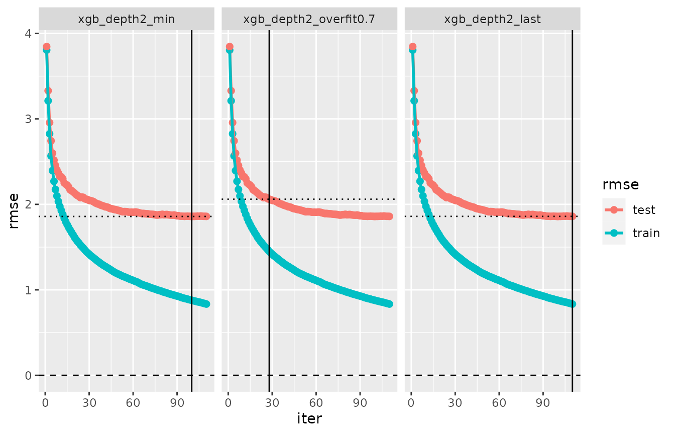

The different structures of cvm_depth2 and cvm_depth2_modif3 also becomes obvious when comparing the respective output from extract_pref_iter():

extract_pref_iter(cvm_depth2)

## Preferred iterations:
##   model 'xgb_depth2':  min (iter=100), overfit0.7 (iter=28), last (iter=110)

extract_pref_iter(cvm_depth2_modif3)

## Preferred iterations:
##   model 'xgb_depth2_min':         min (iter=100)
##   model 'xgb_depth2_overfit0.7':  overfit0.7 (iter=28)
##   model 'xgb_depth2_last':        last (iter=110)

Evaluation log for an alternative metric and `set_metric()`

For the object cv_phe generated above (in the section on “Default metric for xgboost models”), the evaluation log summarizes the training and test errors for all iterations using the default metric, as usual. Here, the default metric is mphe, mean pseudo-Huber error:

evaluation_log(cv_phe) %>% plot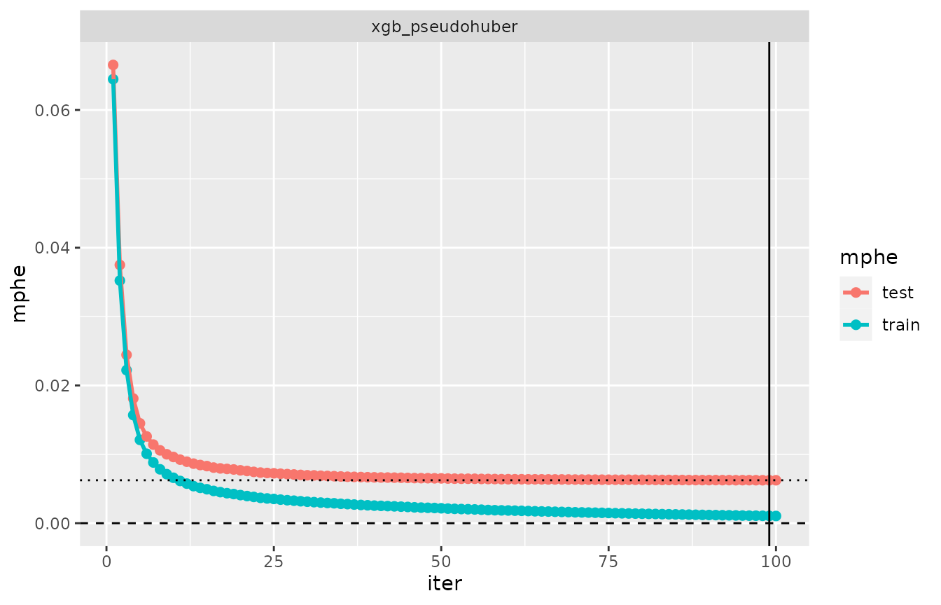

The performance expressed in an alternative metric (for the primary preferred iteration) is obtained with

cv_performance(cv_phe, metric = "mae")

## --- Performance table ---
## Metric: mae
##                 train_mae test_mae iteration time_cv
## xgb_pseudohuber  0.033856 0.081742        99    3.13

The computation of the performance table with a different metric requires the predictions only from the preferred iterations. In contrast, calculation of an evaluation log for a non-default metric requires the predictions from all iterations. As a consequence, the following call won’t produce a useful output (its result is full of NAs):

evaluation_log(cv_phe, metric = "mae")

If the computation of the evaluation log for an alternative metric is required, one can execute the cross-validation setting keep_fits = TRUE in cv(). This saves the fits obtained during cross-validation as a part of the result, such that calculation of predictions from all iterations is possible, thus avoiding having to re-run the cross-validation.

cv_phe_fits <- cv(xgb_phe, keep_fits = TRUE, 
                  folds = cv_phe$folds) # use same folds as in cv_phe
evaluation_log(cv_phe_fits, metric = "mae") %>% plot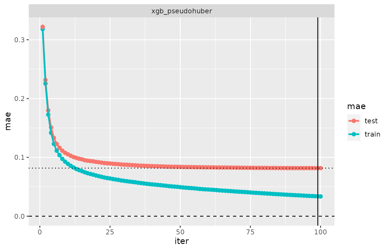

`set_metric()`

The function set_metric() changes the default metric of a “cv” object, thereby computing the evaluation log of the model with that metric. It also re-evaluates the preference criteria such that the preferred iterations may be different from those in the original “cv” object. set_metric() does not re-run a cross-validation, but it requires that the fits are attached to the input “cv”.

cv_phe_mae <- set_metric(cv_phe_fits, "mae")
cv_phe_mae

## --- A "cv" object containing 1 validated model ---
## 
## Validation procedure: Complete k-fold Cross-Validation
##   Number of obs in data:  5000
##   Number of test sets:      10
##   Size of test sets:       500
##   Size of training sets:  4500
## 
## Model:
## 
## 'xgb_pseudohuber':
##   model class:  fm_xgb
##   formula:      log(price) ~ carat + cut + color + clarity + depth + table + x + y + 
##                     z - 1
##   metric:       mae
## 
## Preferred iterations:
##   model 'xgb_pseudohuber':  min (iter=100)

cv_performance(cv_phe_mae)

## --- Performance table ---
## Metric: mae
##                 train_mae test_mae iteration time_cv
## xgb_pseudohuber  0.033588 0.081739       100   3.121

evaluation_log(cv_phe_mae)

## 'evaluation_log', 1 cross-validated model:
## 
## Model 'xgb_pseudohuber':
##   model class: fm_xgb
##  iter train_mae test_mae criterion
##     1    0.3180   0.3220          
##    21    0.0681   0.0918          
##    41    0.0536   0.0850          
##    60    0.0454   0.0831          
##    80    0.0388   0.0821          
##   100    0.0336   0.0817       min

Elastic net: `fm_glmnet()`

In this shorter section on the second class on iteratively fitted models, we use simulated data again. The code below generates a model

\[Y = \beta_1 \cdot X_1 + \beta_2\cdot X_2 + \ldots + \beta_{30}\cdot X_{30} + residual\]

where all \(X_i\) and the residuals are standard normal and \(\beta_i=1/(4i)\) for all \(i\). The beta coefficient are decreasing with \(i\), and we expect that many of them will not have a significant effect on the response \(Y\).

n <- 500; p <- 30
set.seed(1)
x <- matrix(rnorm(n*(p)), n)
beta <- 1/(4*seq(p))
d <- data.frame(y = x%*%beta + rnorm(n), x)
rm(x)

We fit a Lasso model, and run a cross-validation including criteria crit_min() and crit_se(). The usage of the features related to preference criteria and the selection of iterations is exactly as in the xgboost case.

fitted_glmnet <- fm_glmnet(y ~., d)  # glmnet() with default alpha=1: LASSO
plot(fitted_glmnet)  # similar to plot method for class 'glmnet', but a ggplot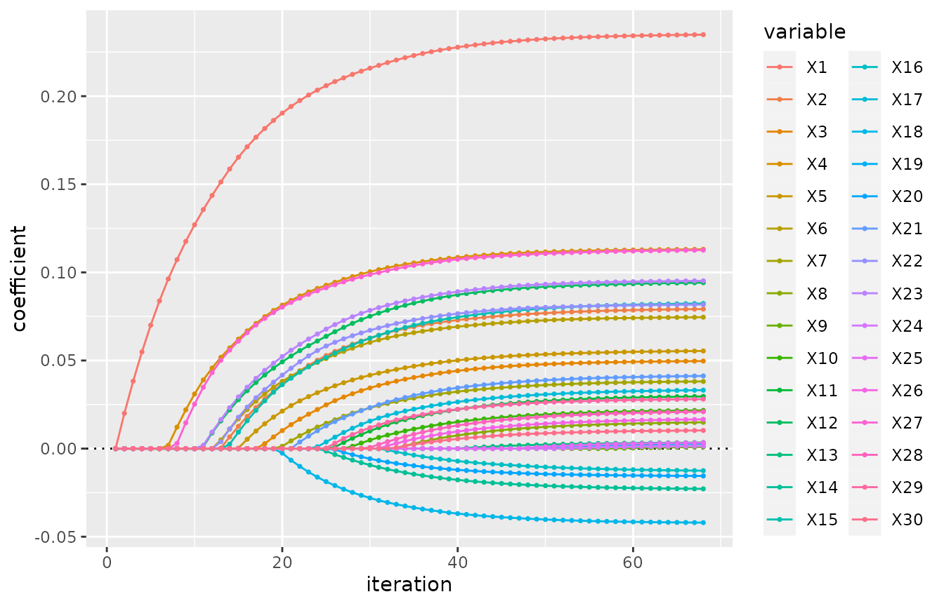

model_glmnet <- model(fitted_glmnet, label = "glmnet")

The application of cv(), cv_performance() and evaluation_log() follows the same logic as for xgboost model:

cv_glmnet <- cv(model_glmnet, iter = c(crit_min(), crit_overfit(.95)))
cv_glmnet

## --- A "cv" object containing 1 validated model ---
## 
## Validation procedure: Complete k-fold Cross-Validation
##   Number of obs in data:  500
##   Number of test sets:     10
##   Size of test sets:       50
##   Size of training sets:  450
## 
## Model:
## 
## 'glmnet':
##   model class:  fm_glmnet
##   formula:      y ~ X1 + X2 + X3 + X4 + X5 + X6 + X7 + X8 + X9 + X10 + X11 + X12 + X13 + 
##                     X14 + X15 + X16 + X17 + X18 + X19 + X20 + X21 + X22 + X23 + X24 + 
##                     X25 + X26 + X27 + X28 + X29 + X30 - 1
##   metric:       rmse
## 
## Preferred iterations:
##   model 'glmnet':  min (iter=19), overfit0.95 (iter=19)

# performance table of cv_glmnet:
cv_performance(cv_glmnet)

## --- Performance table ---
## Metric: rmse
##        train_rmse test_rmse iteration time_cv
## glmnet    0.97368   0.99584        19    0.16

# Plot the evaluation log:
evaluation_log(cv_glmnet) %>% plot(zeroline = FALSE)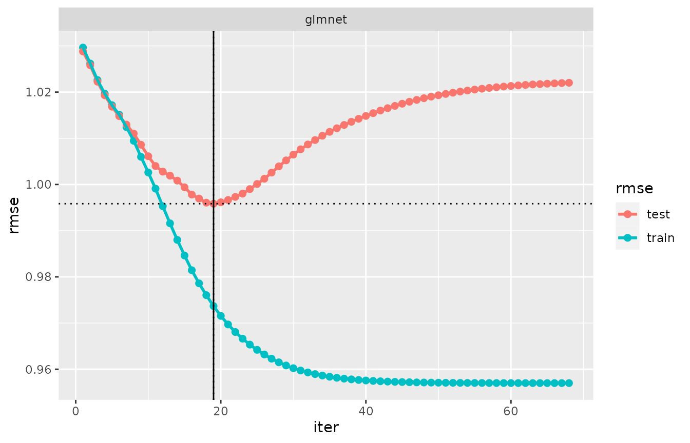

`set_pref_iter()` and `expand_pref_iter()`

Again, the usage of these functions is similar to what has been shown in the section on xgboost models.

set_pref_iter(cv_glmnet, crit_se()) %>% cv_performance # different iteration

## --- Performance table ---
## Metric: rmse
##        train_rmse test_rmse   lambda iteration time_cv
## glmnet    0.97368   0.99584 0.042681        19    0.16

expand_pref_iter(cv_glmnet) %>% cv_performance

## --- Performance table ---
## Metric: rmse
##                    train_rmse test_rmse iteration time_cv
## glmnet_min            0.97368   0.99584        19    0.16
## glmnet_overfit0.95    0.97368   0.99584        19    0.16

Mathias Ambuehl

2023-12-28

Iteratively Fitted Models

The bias-variance trade-off

Boosted trees: `fm_xgb()`

A single model

Evaluation log of a model

Cross-validation

Back to model and fitted model

Tuning `nrounds` with `tune()`

Default metric for xgboost models

Hyperparameter tuning

Cross-validation

`cv_performance()` and `evaluation_log()`

Tuning and extracting a model or fitted model from a “cv” object

Preference criteria for iterations

Basics on preference criteria

Alternative criteria

Specifying a criterion in `cv()`

Back to model and fitted model

Multimodel case

Multiple preference criteria

Changing the primary criterion: `set_pref_iter()`

`expand_pref_iter()`

Evaluation log for an alternative metric and `set_metric()`

`set_metric()`

Elastic net: `fm_glmnet()`

`set_pref_iter()` and `expand_pref_iter()`

Fitting and tuning Iteratively Fitted Models

Mathias Ambuehl

2023-12-28

Iteratively Fitted Models

The bias-variance trade-off

Boosted trees: fm_xgb()

A single model

Evaluation log of a model

Cross-validation

Back to model and fitted model

Tuning nrounds with tune()

Default metric for xgboost models

Hyperparameter tuning

Cross-validation

cv_performance() and evaluation_log()

Tuning and extracting a model or fitted model from a “cv” object

Preference criteria for iterations

Basics on preference criteria

Alternative criteria

Specifying a criterion in cv()

Back to model and fitted model

Multimodel case

Multiple preference criteria

Changing the primary criterion: set_pref_iter()

expand_pref_iter()

Evaluation log for an alternative metric and set_metric()

set_metric()

Elastic net: fm_glmnet()

set_pref_iter() and expand_pref_iter()

Boosted trees: `fm_xgb()`

Tuning `nrounds` with `tune()`

`cv_performance()` and `evaluation_log()`

Specifying a criterion in `cv()`

Changing the primary criterion: `set_pref_iter()`

`expand_pref_iter()`

Evaluation log for an alternative metric and `set_metric()`

`set_metric()`

Elastic net: `fm_glmnet()`

`set_pref_iter()` and `expand_pref_iter()`