Plot method for class “evaluation_log”
plot.evaluation_log.RdDraws line plots of training and test errors in an evaluation log, if available.
Arguments
- x
An object of class
evaluation_log.- errorbars
Logical: Whether to add error bars in plots.
- plot
Logical: If
TRUE, a ggplot is returned, ifFALSEadata.frame.plot()first prepares adata.frameand then draws some ggplot using this data, with limited options for customization. If you want to design your own plot, you can setplot=FALSE, and use thedata.framereturned byplot()to create your plot.- size
Graphic detail: Size of point.
- lwd
Graphic detail: Line width of interpolating line.
- lwd_errorbars
Graphic detail: Line width of errorbars.
- zeroline
Logical: Whether to include a horizontal reference line at level 0.
- ...
Currently not used.
Value
plot.evaluation_log() returns either a ggplot or, if plot=FALSE, a data.frame.
Examples
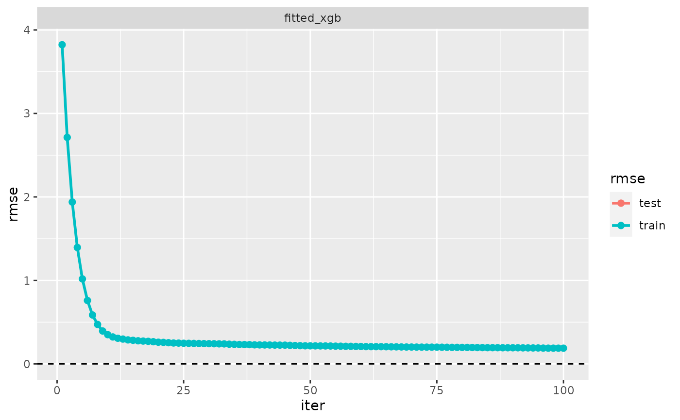
# Evaluation log of a 'fm_xgb' model
fitted_xgb <- fm_xgb(Sepal.Length ~ ., iris, max_depth = 2)
evaluation_log(fitted_xgb) # evaluation log of a model has no
#> ‘evaluation_log’, 1 model:
#>
#> Model ‘fitted_xgb’:
#> model class: fm_xgb
#> iter train_rmse test_rmse
#> 1 3.823 NA
#> 21 0.258 NA
#> 41 0.227 NA
#> 60 0.209 NA
#> 80 0.197 NA
#> 100 0.188 NA
plot(evaluation_log(fitted_xgb))
#> Warning: Removed 100 rows containing missing values (`geom_point()`).
#> Warning: Removed 100 rows containing missing values (`geom_line()`).
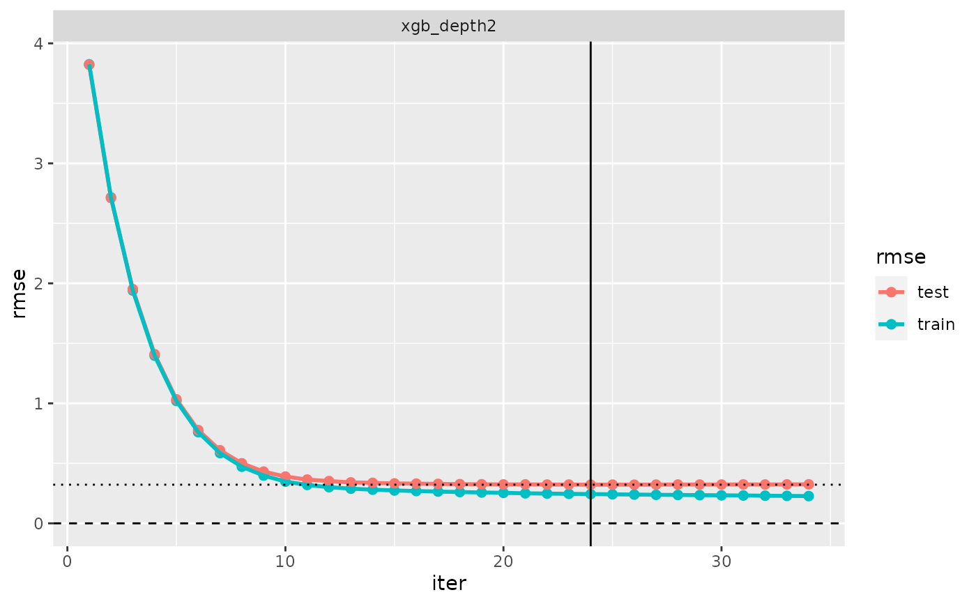
 # Evaluation log of cross-validated 'fm_xgb' model
cv_xgb <- cv(model(fitted_xgb, label = "xgb_depth2"))
evaluation_log(cv_xgb)
#> ‘evaluation_log’, 1 cross-validated model:
#>
#> Model ‘xgb_depth2’:
#> model class: fm_xgb
#> iter train_rmse test_rmse criterion
#> 1 3.825 3.821
#> 8 0.472 0.500
#> 14 0.280 0.337
#> 21 0.250 0.325
#> 24 0.244 0.322 min
#> 27 0.238 0.323
#> 34 0.227 0.325
plot(evaluation_log(cv_xgb))
# Evaluation log of cross-validated 'fm_xgb' model
cv_xgb <- cv(model(fitted_xgb, label = "xgb_depth2"))
evaluation_log(cv_xgb)
#> ‘evaluation_log’, 1 cross-validated model:
#>
#> Model ‘xgb_depth2’:
#> model class: fm_xgb
#> iter train_rmse test_rmse criterion
#> 1 3.825 3.821
#> 8 0.472 0.500
#> 14 0.280 0.337
#> 21 0.250 0.325
#> 24 0.244 0.322 min
#> 27 0.238 0.323
#> 34 0.227 0.325
plot(evaluation_log(cv_xgb))
 # Evaluation log of several cross-validated models
mydata <- simuldat()
fitted_glmnet <- fm_glmnet(Y ~ ., mydata)
cv_glmnet <- cv(multimodel(fitted_glmnet, prefix = "glmnet", alpha = 0:1))
label(cv_glmnet) <- c("ridge", "lasso")
evaluation_log(cv_glmnet)
#> ‘evaluation_log’, 2 cross-validated models:
#>
#> Model ‘ridge’:
#> model class: fm_glmnet
#> iter lambda train_rmse test_rmse criterion
#> 1 1039.726 2.76 2.75
#> 21 161.748 2.74 2.73
#> 41 25.163 2.62 2.62
#> 60 4.296 2.25 2.30
#> 80 0.668 1.93 2.04
#> 92 0.219 1.90 2.03 min
#> 100 0.104 1.89 2.03
#>
#> Model ‘lasso’:
#> model class: fm_glmnet
#> iter lambda train_rmse test_rmse criterion
#> 1 1.03973 2.76 2.76
#> 14 0.31022 2.18 2.20
#> 27 0.09256 1.95 2.05
#> 40 0.02762 1.90 2.03
#> 44 0.01903 1.90 2.03 min
#> 53 0.00824 1.89 2.03
#> 66 0.00246 1.89 2.03
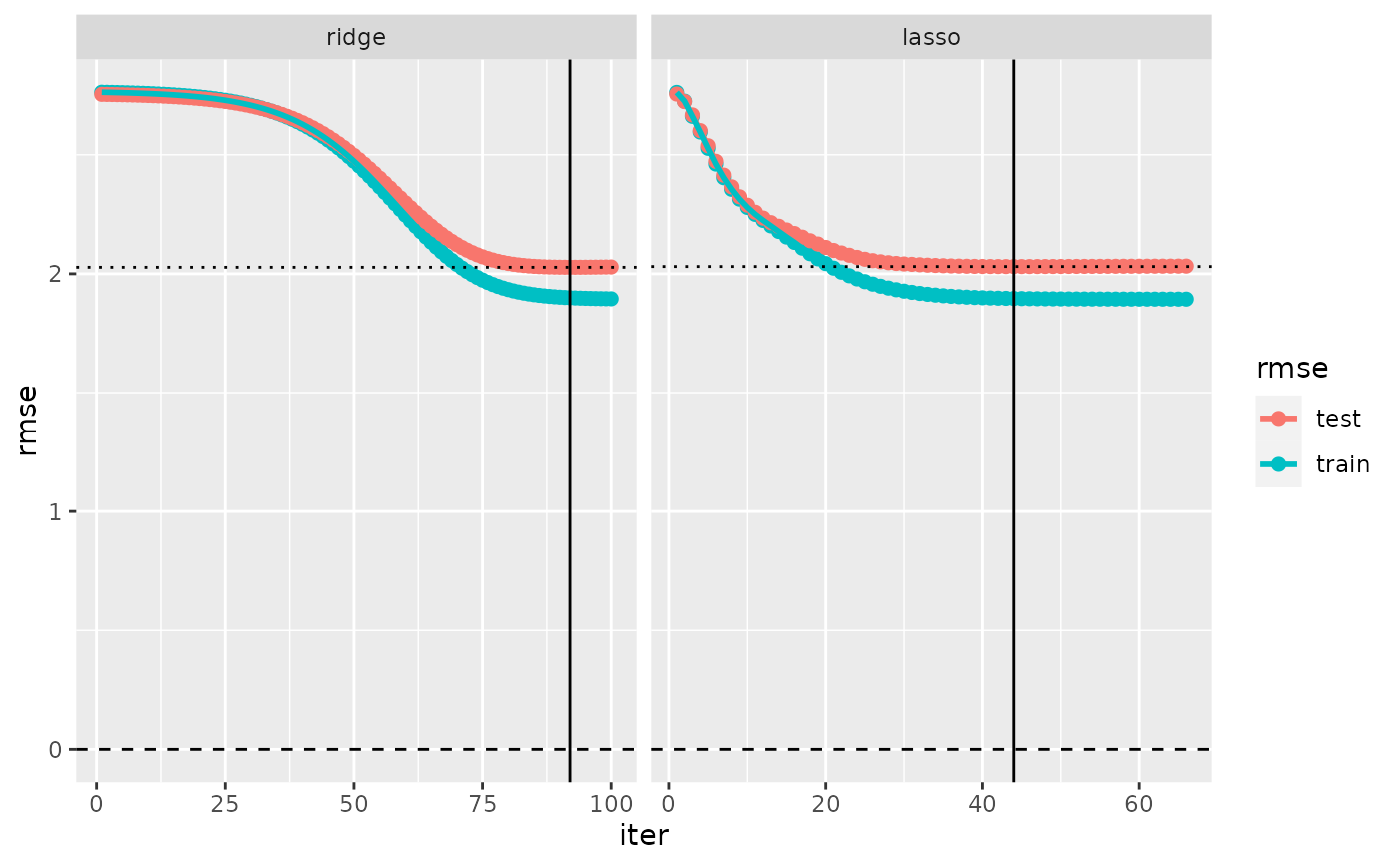
plot(evaluation_log(cv_glmnet))
# Evaluation log of several cross-validated models
mydata <- simuldat()
fitted_glmnet <- fm_glmnet(Y ~ ., mydata)
cv_glmnet <- cv(multimodel(fitted_glmnet, prefix = "glmnet", alpha = 0:1))
label(cv_glmnet) <- c("ridge", "lasso")
evaluation_log(cv_glmnet)
#> ‘evaluation_log’, 2 cross-validated models:
#>
#> Model ‘ridge’:
#> model class: fm_glmnet
#> iter lambda train_rmse test_rmse criterion
#> 1 1039.726 2.76 2.75
#> 21 161.748 2.74 2.73
#> 41 25.163 2.62 2.62
#> 60 4.296 2.25 2.30
#> 80 0.668 1.93 2.04
#> 92 0.219 1.90 2.03 min
#> 100 0.104 1.89 2.03
#>
#> Model ‘lasso’:
#> model class: fm_glmnet
#> iter lambda train_rmse test_rmse criterion
#> 1 1.03973 2.76 2.76
#> 14 0.31022 2.18 2.20
#> 27 0.09256 1.95 2.05
#> 40 0.02762 1.90 2.03
#> 44 0.01903 1.90 2.03 min
#> 53 0.00824 1.89 2.03
#> 66 0.00246 1.89 2.03
plot(evaluation_log(cv_glmnet))